Purpose
Return value
Syntax
=AGGREGATE(function_num,options,ref1,[ref2],...)- function_num - Operation to perform (1-19).
- options - Values to ignore (0-7).
- ref1 - First argument.
- ref2 - [optional] Second argument (k).
Using the AGGREGATE function
The AGGREGATE function returns the result of an aggregate calculation like AVERAGE, COUNT, MAX, MIN, etc. performed on one or more references. The AGGREGATE function is like an upgraded version of the older SUBTOTAL function, and provides more calculation options, and more control over ignoring specific things. There are two reasons that make the AGGREGATE function especially useful, compared to other functions which perform the same operations:
- AGGREGATE has a number of options for ignoring errors, hidden rows, and other functions that may appear in data.
- AGGREGATE can handle many array operations natively, without Control + Shift + Enter.
AGGREGATE can run a total of 19 functions, and the function to perform is given as a number, which appears as the first argument in the function, function_num. The second argument, options, controls how AGGREGATE handles errors and values in hidden rows. See the table below for all available options.
The AGGREGATE function takes four arguments: function_num, options, ref1, and ref2. For the first 13 functions supported, only the first three arguments are required: function_num specifies the operation, options controls various behaviors, and ref1 is the array of values to process.
The last 6 functions require all four arguments: function_num specifies the operation, options controls various behaviors, ref1 is the array of values to process, and ref2 is the "second argument" for the function being called. For example, functions like SMALL and LARGE take a second argument, k, and ref2 represents that argument. The following six functions require the ref2 argument:
LARGE(array,k)
SMALL(array,k)
PERCENTILE.INC(array,k)
QUARTILE.INC(array,quart)
PERCENTILE.EXC(array,k)
QUARTILE.EXC(array,quart)
Example #1
To return the MAX value in the range A1:A10, ignoring both errors and hidden rows, provide 4 for function number and 7 for options:
=AGGREGATE(4,7,A1:A10) // max value
To return the MIN value with the same options, change the function number to 5:
=AGGREGATE(5,7,A1:A10) // min value
Example #2
In the example shown above, the formula in D5 is:
=AGGREGATE(4,6,values)
where "values" is the named range B5:B14. The function number is 4, which specifies MAX. Options is provided as 6, to ignore errors only.
Example #3 - nth largest
The formulas in D8:D10 demonstrate how to return "nth largest" values:
=AGGREGATE(14,6,values,1) // 1st largest
=AGGREGATE(14,6,values,2) // 2nd largest
=AGGREGATE(14,6,values,3) // 3rd largest
The function number here is 14, which runs the LARGE function. Because the LARGE function requires a k argument, it appears as the last argument in the three formulas above.
Example #4 - array operation
What makes AGGREGATE especially useful for more complex formulas is that it can handle arrays natively when the function number is 14-19. For example, to find the MAX value on Mondays, with data that includes dates and values, you could use AGGREGATE like this:
=AGGREGATE(14,6,values/(TEXT(dates,"ddd")="Mon"),1)
Here we specify 14 for function (LARGE) and 6 for option (ignore errors). Then we build a logical expression using the TEXT function to check all dates for Mondays. The result of this operation is an array of TRUE/FALSE values, which become the denominator of the original values. FALSE evaluates as zero, and throws a #DIV/0! error. TRUE evaluates as 1 and returns the original value. The final array of values and errors acts like a filter. AGGREGATE ignores all errors and returns the largest (maximum) of the surviving values. More complete example here.
Function numbers
The table below lists the function numbers available to the AGGREGATE function, along with the name of the associated function. The third column, Ref2, indicates the "second argument" expected by the last 6 functions.
| Function number | Function | Ref2 |
|---|---|---|
| 1 | AVERAGE | |
| 2 | COUNT | |
| 3 | COUNTA | |
| 4 | MAX | |
| 5 | MIN | |
| 6 | PRODUCT | |
| 7 | STDEV.S | |
| 8 | STDEV.P | |
| 9 | SUM | |
| 10 | VAR.S | |
| 11 | VAR.P | |
| 12 | MEDIAN | |
| 13 | MODE.SNGL | |
| 14 | LARGE | k |
| 15 | SMALL | k |
| 16 | PERCENTILE.INC | k |
| 17 | QUARTILE.INC | quart |
| 18 | PERCENTILE.EXC | k |
| 19 | QUARTILE.EXC | quart |
Behavior options
The AGGREGATE function has many options for ignoring errors, hidden rows, and other functions. Options are set with the options argument. Possible values are 0-7, as shown in the table below.
| Option | Behavior |
|---|---|
| 0 | Ignore SUBTOTAL and AGGREGATE functions |
| 1 | Ignore hidden rows, SUBTOTAL and AGGREGATE functions |
| 2 | Ignore error values, SUBTOTAL and AGGREGATE functions |
| 3 | Ignore hidden rows, error values, SUBTOTAL and AGGREGATE functions |
| 4 | Ignore nothing |
| 5 | Ignore hidden rows |
| 6 | Ignore error values |
| 7 | Ignore hidden rows and error values |
Note: The AGGREGATE function is like an upgraded version of the older SUBTOTAL function, and provides more calculation options, and more control over ignoring specific things. However, one subtle difference between AGGREGATE and SUBTOTAL is that the default behavior for hidden rows is reversed. While SUBTOTAL will always ignore values in rows hidden by a filter, and needs a different function number to ignore manually hidden rows, AGGREGATE will always ignore manually hidden rows and needs a specific option to ignore rows hidden by a filter. Even when the option argument is set to 4 (ignore nothing), AGGREGATE will ignore values in manually hidden rows.
Notes
- AGGREGATE returns a #VALUE! error if a second function argument is required, but not provided.
- 3D references do not work with AGGREGATE.
- The AGGREGATE function is designed for vertical ranges, not horizontal ranges.


