Summary
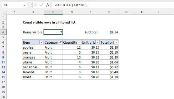
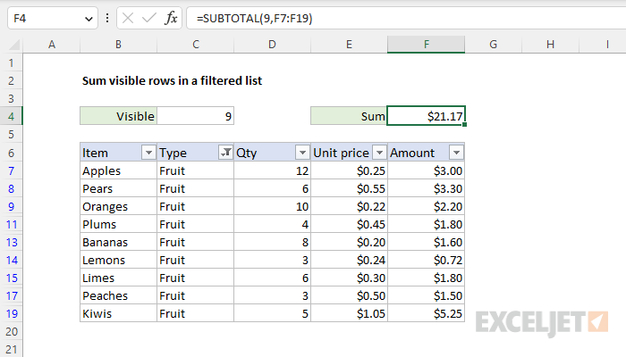
To sum values in visible rows in a filtered list (i.e. exclude rows that are "filtered out"), you can use the SUBTOTAL function. In the example shown, the formula in F4 is:
=SUBTOTAL(9,F7:F19)
The result is $21.17, the sum of the 9 visible values in column F. Note that the range F7:F19 contains 13 values total, 4 of which are hidden by the filter in column C.
Generic formula
=SUBTOTAL(9,range)
Explanation
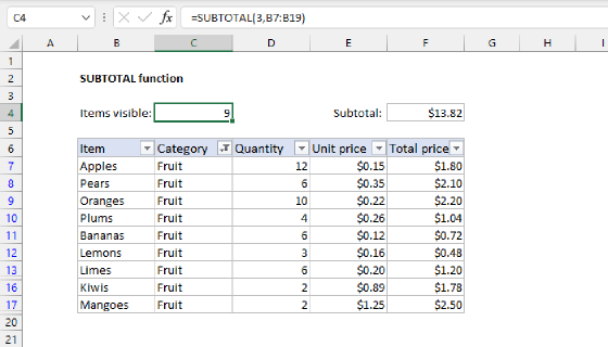
In this example, the goal is to sum values in rows that are visible and ignore values in rows that are hidden. The range F7:F19 contains 13 values total, 4 of which are hidden by the filter applied to column C. This is a good job for the SUBTOTAL function, which can distinguish between visible and hidden cells when it applies various calculations. Another way to solve this problem is with the AGGREGATE function. Both formulas are explained below.
SUBTOTAL function
The SUBTOTAL function can perform a variety of calculations like COUNT, SUM, MAX, MIN, etc. on a set of data, returning an aggregated result. What makes SUBTOTAL useful in this case is that it will automatically ignore rows that are hidden in a filtered list or table and can optionally ignore rows that have been manually hidden. The generic syntax for SUBTOTAL looks like this:
=SUBTOTAL(function_num, reference)
The first argument, function_num, specifies the type of calculation to perform. Reference holds the data that should be used in the operation. In the worksheet shown above, we use SUBTOTAL like this:
=SUBTOTAL(9,F7:F19) // sum and ignore hidden
For function_num, we provide the number 9, which corresponds to the "SUM" operation. For reference, we use the full range for the amounts in column F, which is F7:F19. SUBTOTAL automatically ignores the 4 rows hidden by the filter applied to column C, and returns $21.17, the sum of the 9 visible amounts in column F.
Note that SUBTOTAL always ignores values in rows that are hidden with a filter. To ignore rows that are hidden manually (i.e. right-click > Hide), use 109 for function_num instead of 9:
=SUBTOTAL(109,B7:B16) // sum and ignore manually hidden
To be clear, SUBTOTAL will always ignore values in rows hidden by a filter in a table, regardless of function_num. Using 109 instead of 9 simply changes the behavior to also ignore manually hidden rows. SUBTOTAL function can perform many other calculations as well. See a complete list on this page.
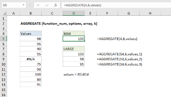
AGGREGATE function
The AGGREGATE function is like an ungraded version of SUBTOTAL. Like SUBTOTAL, AGGREGATE can run many aggregate calculations, optionally ignoring hidden rows. However, AGGREGATE provides more calculation options, and more options for ignoring things. The formulas below show how AGGREGATE can be used like the SUBTOTAL function to solve this problem:
=AGGREGATE(9,5,F7:F19) // sum, ignore hidden
=AGGREGATE(9,7,F7:F19) // sum, ignore hidden and errors
The second formula shows how to configure AGGREGATE to ignore hidden rows and errors in the data at the same time. AGGREGATE provides a total of 19 different calculations and many options for ignoring things. For details, see our AGGREGATE function page.
Note: One subtle difference between AGGREGATE and SUBTOTAL is that default behavior for hidden rows is reversed. While SUBTOTAL will always ignore values in rows hidden by a filter, and needs a different function number to ignore manually hidden rows, AGGREGATE will always ignore manually hidden rows and needs a specific option to ignore rows hidden by a filter.