Summary
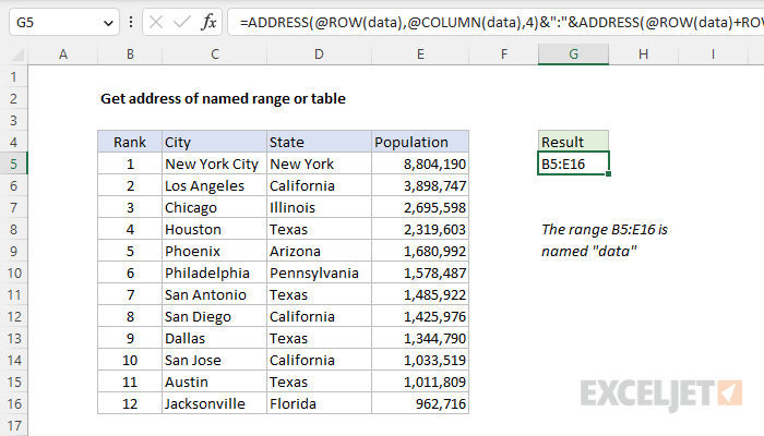
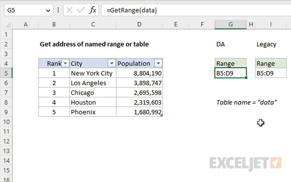
To get the address of a named range or an Excel Table as text, you can use the ADDRESS function. In the example shown, the formula in G5 is:
=ADDRESS(@ROW(data),@COLUMN(data),4)&":"&ADDRESS(@ROW(data)+ROWS(data)-1,@COLUMN(data)+COLUMNS(data)-1,4)
where data is the named range B5:E16.
Note: Excel 365 requires the implicit intersection operator (@) as shown above. In Legacy Excel, this is not necessary. See below for a more elegant solution that takes advantage of dynamic array formulas.
Generic formula
=ADDRESS(ROW(name),COLUMN(name))&":"&ADDRESS(ROW(name)+ROWS(name)-1,COLUMN(name)+COLUMNS(name)-1)
Explanation
The goal is to return the full address of a range or named range as text. The purpose of this formula is informational, not functional. It provides a way to inspect the current range for a named range, an Excel Table, or even the result of a formula. The core of the solutions explained below is the ADDRESS function, which returns a cell address based on a given row and column. The formula gets somewhat complicated because we need to use ADDRESS twice, and because there is a lot of busy work in collecting the coordinates we need to provide to ADDRESS. See below for a more elegant formula that takes advantage of the LET function and the TAKE function in Excel 365. This version can also report the range returned by another function (like OFFSET).
Note: the CELL function is another way to get the address for a cell. However, CELL does not provide a way to choose a relative or absolute format like the ADDRESS function does. In addition, CELL is a volatile function and can cause performance problems in large or complex worksheets. For those reasons, I have avoided it in this example.
Background
The links below provide more details about Excel Tables and named ranges:
- How to create an Excel Table (video)
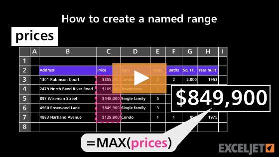
- How to create a named range (video)
- How to create a dynamic named range with a table (video)
Demo
The animation below shows how the formula responds when a Table named "data" is resized. In the worksheet, DA stands for Dynamic Array version of Excel and Legacy stands for older versions of Excel. See below for more information about the dynamic array version.
The basic idea
The basic idea of this formula is to get the coordinates of the first (upper left) cell in a range and the last (lower right) cell in a range, then use these coordinates to create cell references, then join the references together with concatenation. The formula itself looks complicated and scary:
=ADDRESS(@ROW(data),@COLUMN(data),4)&":"&ADDRESS(@ROW(data)+ROWS(data)-1,@COLUMN(data)+COLUMNS(data)-1,4)
However, most of what you see is the "busy work" of collecting the coordinates with the ROW, ROWS, COLUMN, and COLUMNS functions. Once that work is done, the formula simplifies to this:
=ADDRESS(5,2,4)&":"&ADDRESS(16,4,4)
The ADDRESS function then creates a reference to the first and last cell in the range, and the two references are joined together. That's it. The rest of the problem is the details of collecting the coordinates needed by the ADDRESS function.
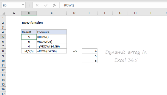
ROW and COLUMN functions
The ROW and COLUMN functions simply return coordinates. For example, if we give ROW and COLUMN cell B5 as a reference, we get back coordinate numbers:
=ROW(B5) // returns 5
=COLUMN(B5) // returns 2
Notice that COLUMN returns a number, not a letter: column A, is 1, column B is 2, column C is 3, etc.
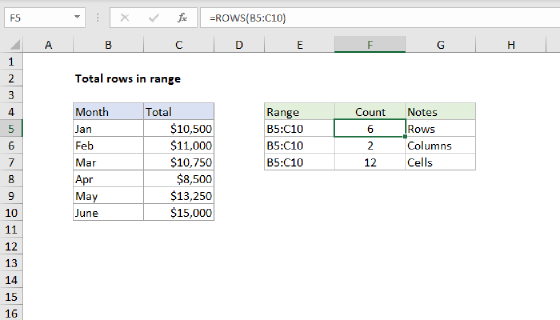
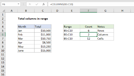
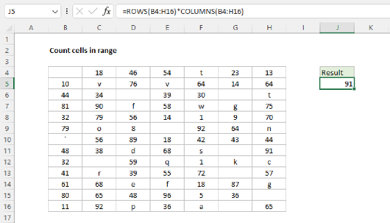
ROWS and COLUMNS functions
The ROWS and COLUMNS functions return counts. For example, if we give ROWS and COLUMNS the range B5:D16, we get back the number of rows and the number of columns in the range:
=ROWS(B5:D16) // returns 12
=COLUMNS(B5:D16) // returns 3
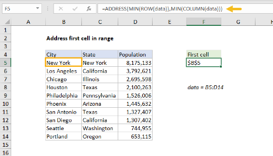
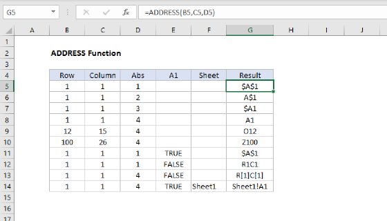
ADDRESS function
The ADDRESS function returns the address for a cell based on a given row and column number as text. For example:
=ADDRESS(1,1) // returns "$A$1"
=ADDRESS(5,2) // returns "$B$5"
Note that ADDRESS returns an address as an absolute reference by default. However, by providing 4 for the optional argument abs_num, ADDRESS will return a relative reference:
=ADDRESS(1,1,4) // returns "A1"
=ADDRESS(5,2,4) // returns "B5"
In this problem, we need to build up an address for a range in two parts (1) a reference to the first cell in the range and (2) a reference to the last cell in a range. To get the address for the first cell in the range, we use this formula:
=ADDRESS(@ROW(data),@COLUMN(data))
Note: data is the named range B5:E16.
As mentioned above, the ROW function and the COLUMN function return coordinates: ROW returns a row number, and COLUMN returns a column number. In this case however, we are giving ROW and COLUMN the range data, not a single cell. As a result, we get back an array of numbers:
=ROW(data) // returns {5;6;7;8;9;10;11;12;13;14;15;16}
=COLUMN(data) // returns {2,3,4,5}
In other words, ROW returns all row numbers for data (B5:D15), and COLUMN returns all column numbers for data. This is where the formula gets a bit complicated due to Excel version differences.
Although ROW and COLUMN return multiple results, older versions of Excel will automatically limit the results to the first value only. This works fine for the problem at hand, because we only want the first value. However, in the dynamic version of Excel, multiple results are not automatically limited, because formulas can spill results onto the worksheet. We don't want this behavior in this case, so we use the implicit intersection operator (@) to limit the output from ROW and COLUMN to one value only:
=@ROW(data) // returns 5
=@COLUMN(data) // returns 2
In effect, this mimics the behavior in Legacy Excel where formulas that return more than one result display one result only. Note that the implicit intersection operator (@) is not required in Legacy Excel. In fact, if you try to add the @ in an older version of Excel, Excel will simply remove it. However, it is required in the current version of Excel.
Returning to the formula, ROW and COLUMN return their results directly to ADDRESS as the row_num and column_num arguments. With abs_num provided as 4 (relative), ADDRESS returns the text "B5".
=ADDRESS(5,2,4) // returns "B5"
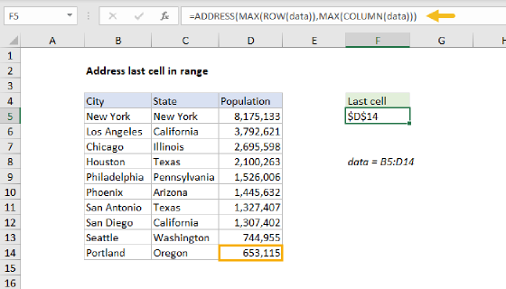
To get the last cell in the range, we use the ADDRESS function again like this:
ADDRESS(@ROW(data)+ROWS(data)-1,@COLUMN(data)+COLUMNS(data)-1,4)
Essentially, we follow the same idea as above, using ROW and COLUMN to get the last row and last column of the range. However, we also calculate the total number of rows with the ROWS function and the total number of columns with the COLUMNS function:
=ROWS(data) // returns 12
=COLUMNS(data) // returns 4
Then we do some simple math to calculate the row and column number of the last cell. We add the row count to the starting row, and add the column count to the starting column, then subtract 1 to get the correct coordinates for the last cell:
=ADDRESS(@ROW(data)+ROWS(data)-1,@COLUMN(data)+COLUMNS(data)-1,4)
=ADDRESS(5+12-1,2+4-1,4)
=ADDRESS(16,5,4)
="E16"
With abs_num set to 4. ADDRESS returns "E16", the address of the last cell in data as text. At this point, we have the address for the first cell and the address for the last cell. The only thing left to do is concatenate them together separated by a colon:
="B5"&":"&"E16"
="B5:E16"
More elegant formula
Although the formula above works fine, it is cumbersome and redundant. New array functions in Excel make it possible to solve the problem with a more elegant formula like this:
=LET(
first,TAKE(rng,1,1),
last,TAKE(rng,-1,-1),
ADDRESS(ROW(first),COLUMN(first),4)&":"&
ADDRESS(ROW(last),COLUMN(last),4)
)
Where rng is the generic placeholder for a named range or Excel Table. In this formula, the LET function is used to assign values to two variables: first and last. First represents the first cell in the range and last represents the last cell in the range. These values are assigned with the TAKE function like this:
first,TAKE(rng,1,1), // first cell (B5)
last,TAKE(rng,-1,-1), // last cell (E16)
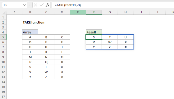
The TAKE function returns a subset of a given array or range. The size of the array returned is determined by separate rows and columns arguments. When positive numbers are provided for rows or columns, TAKE returns values from the start or top of the array. Negative numbers take values from the end or bottom of the array. What's tricky about this, and not obvious, is that when working with ranges, TAKE returns a valid reference. You don't normally see the reference because as with most formulas, Excel returns the value at that reference, not the reference itself. However, the reference is there, as is obvious in the next step.
Finally, the ADDRESS function is used to generate an address for both the first cell and the last cell in the range, and the two results are concatenated with a colon (:) in between:
ADDRESS(ROW(first),COLUMN(first),4)&":"&ADDRESS(ROW(last),COLUMN(last),4)
Substituting the references returned by TAKE, the formula evaluates like this:
=ADDRESS(ROW(B5),COLUMN(B5),4)&":"&ADDRESS(ROW(E16),COLUMN(E16),4)
=ADDRESS(5,2,4)&":"&ADDRESS(16,4,4)
="B5"&":"&"E16"
="B5:E16"
Named range as text
To get an address for a named range entered as a text value (i.e. "range", "data", etc.), you'll need to use the INDIRECT function to change the text into a valid reference before proceeding. For example, to get the address of a table name entered in A1 as text, you could use this unwieldy formula:
=ADDRESS(ROW(INDIRECT(A1)),COLUMN(INDIRECT(A1)))&":"&ADDRESS(ROW(INDIRECT(A1))+ROWS(INDIRECT(A1))-1,COLUMN(INDIRECT(A1))+COLUMNS(INDIRECT(A1))-1)
In the dynamic array version of Excel, the LET function makes this much simpler. With a range or table name as text in cell A1, you can call INDIRECT just once like this:
=LET(
rng,INDIRECT(A1),
first,TAKE(rng,1,1),
last,TAKE(rng,-1,-1),
ADDRESS(ROW(first),COLUMN(first),4)&":"&
ADDRESS(ROW(last),COLUMN(last),4)
)
You can read more about the LET function here.
Named LAMBDA option
Taking things a step further, you can use the LAMBDA function to create a custom function like this:
=LAMBDA(range,
  LET(
    rng,IF(ISREF(range),range,INDIRECT(range)),
    first,TAKE(rng,1,1),
    last,TAKE(rng,-1,-1),
    ADDRESS(ROW(first),COLUMN(first),4)&":"&
    ADDRESS(ROW(last),COLUMN(last),4)
  )
)(data)
This version of the formula does the same thing as the formula above with one additional step: it checks for range or table names entered as text values. This is done with the ISREF function in the first step. If the value passed in for range is a valid reference, we use it as-is to assign a value to rng. If not, we run it through the INDIRECT function to try and get a valid reference.
Finally, if we give the LAMBDA formula above the name "GetRange", we can call it on any valid range like this:
=GetRange(data)
Read more about creating and naming custom LAMBDA formulas here.
Check reference returned by formula
A nice feature of the LAMBDA version of the formula is we easily can use it to check the result of any formula that returns a range. For example, we can call it with the OFFSET function like this:
=GetRange(OFFSET(A1,4,1,10,2)) // returns "B5:C14"
The point here is that it is not easy to understand what range is returned by OFFSET, because Excel will return only the values in the range. The custom GetRange function makes it possible to print the range returned by a formula explicitly.
Other ideas
I looked at two other formulas to solve this problem. The first uses ADDRESS and TAKE:
=LET(
a,ADDRESS(ROW(data),COLUMN(data),4),
TAKE(a,1,1)&":"&TAKE(a,-1,-1)
)
The second uses ADDRESS and the new TOCOL function:
=LET(
a,TOCOL(ADDRESS(ROW(data),COLUMN(data),4)),
INDEX(a,1)&":"&INDEX(a,ROWS(d))
)
Both formulas use the ADDRESS function to spin up all of the addresses in the range at the same time. The first formula then uses the TAKE function to get the first and last address. The second formula uses the TOCOL function to unwrap the array of references created by ADDRESS, then it uses the INDEX function twice to get the first and the last value. On small ranges, these formulas should work nicely. However, on very large ranges you are likely to see a performance hit because of the time needed to create all of the extra addresses. The proposed formula solution above avoids this problem by only creating the first and last reference. The tradeoff is that the formula is more complex.