Explanation
The ADDRESS function creates a reference based on a given a row and column number. In this case, we want to get the last row and the last column used by the named range data (B5:D14).
To get the last row used, we use the ROW function together with the MAX function like this:
MAX(ROW(data))
Because data contains more than one row, ROW returns an array of row numbers:
{5;6;7;8;9;10;11;12;13;14}
This array goes directly to the MAX function, which returns the largest number:
MAX({5;6;7;8;9;10;11;12;13;14}) // returns 14
To get the last column, we use the COLUMN function in the same way:
MAX(COLUMN(data))
Since data contains three rows, COLUMN returns an array with three column numbers:
{2,3,4}
and the MAX function again returns the largest number:
MAX({2,3,4}) // returns 4
Both results are returned directly to the ADDRESS function, which constructs a reference to the cell at row 14, column 4:
=ADDRESS(14,4) // returns $D$14
If you want a relative address instead of an absolute reference, you can supply 4 for the third argument like this:
=ADDRESS(MAX(ROW(data)),MAX(COLUMN(data)),4) // returns D14
CELL function alternative
Although it's not obvious, the INDEX function returns a reference, so we can use the CELL function with INDEX to get the address of the last cell in a range like this:
=CELL("address",INDEX(data,ROWS(data),COLUMNS(data)))
In this case, we use the INDEX function to get a reference to the last cell in the range, which we determine by passing total rows and total columns for the range data into INDEX. We get total rows with the ROWS function, and total columns with the COLUMNS function:
ROWS(data) // returns 10
COLUMNS(data) // returns 3
With the array provided as data, INDEX then returns a reference to cell D14:
INDEX(data,10,3) // returns reference to D14
We then use the CELL function with "address", to display the address.
Note: The CELL function is a volatile function which can cause performance problems in large or complex workbooks.


