Summary
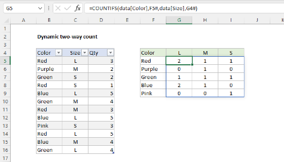
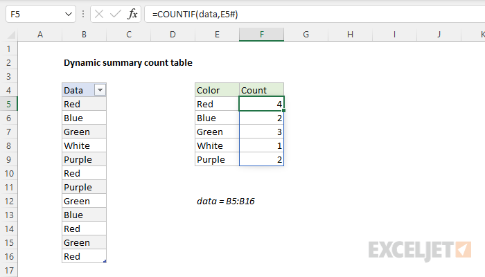
To create a basic dynamic summary count with a formula, you can use the UNIQUE function to get unique values, and the COUNTIF function to count those values in the data. In the example shown, the formula in F5 is:
=COUNTIF(data,E5#)
Where data is an Excel Table in B5:B16. With five values in E5:E9, COUNTIF returns the five counts to cell F5, and the results spill into the range F5:F9. See below for progressively more advanced options including all-in-one formulas.
Explanation
In this example, the goal is to build a simple summary count table with a formula. Once created, the summary table should automatically update to show new values and counts when data changes. The article below walks through several options, from simple to very advanced. The more advanced options show how to sort the table in descending order by count.
Manual formula
Note that it is possible to build a summary table with formulas manually. The basic approach is to copy all values, use the Remove Duplicates command to get unique values, and then copy a COUNTIF formula into each cell that needs to show a count:
Video: How to build a simple summary table
This works fine, but the summary table will not update automatically if new values are added or removed from the data. In other words, if a new color is added to the data table, it will not appear in the summary table.
Pivot table
Another good approach is to use a Pivot Table. This is one of the easiest ways to create a summary count, and if you use an Excel Table as the source data, the summary will stay in sync with the data. Also, the summary table can be easily sorted in a Pivot Table. However, a Pivot Table must be refreshed to see the latest data, and the solution is not a formula. Nevertheless, a pivot table is an excellent way to create a summary table.
Video: How to quickly create a pivot table
Two formulas
In the dynamic array version of Excel, a simple way to create a summary table is to use two formulas, one to collect unique values, and one to count the values. This is the solution shown in the worksheet at the top of the page. The formula in E5 is based on the UNIQUE function:
=UNIQUE(data) // get unique values
The formula in F5 uses the COUNTIF function:
=COUNTIF(data,E5#) // count unique values
Notice that inside COUNTIF, the table named data is provided as the range argument, and the spill reference E5# is used for criteria. When source data changes, both formulas will stay in sync. In general this is a good, simple option. However, there are limitations. For example, because there are two separate formulas, we can't sort the results (in place) with the SORT function.
All-in-one formula
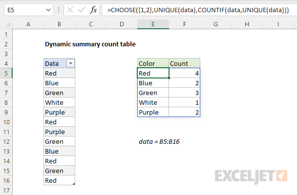
A more advanced solution involves an all-in-one formula. One approach looks like this:
=CHOOSE({1,2},UNIQUE(data),COUNTIF(data,UNIQUE(data)))
In this formula, we are using the CHOOSE function to combine two arrays. The first array contains the unique values in the data:
UNIQUE(data) // unique values
The second array is essentially the COUNTIF formula explained above, except the criteria argument is created dynamically:
COUNTIF(data,UNIQUE(data)) // counts
Note: we are using CHOOSE function as a stand-in for the forthcoming HSTACK function, which has just been released to the Beta Channel.
The CHOOSE function combines both arrays into a single array, which displays as a two-column table in the worksheet:
Sorting results
Now that we have a formula that returns the entire table, we can easily sort the table in descending order by count. To do this, we wrap the entire formula in the SORT function, and specify 2 for sort_index and -1 for sort_order:
=SORT(CHOOSE({1,2},UNIQUE(data),COUNTIF(data,UNIQUE(data))),2,-1)
Video: Basic SORT function example
Now the table will update automatically if data changes, and the table will remain sorted by count, with highest counts at the top.
With the LET function
We can use the LET function to streamline the formula a bit, by defining a variable, u, to hold the unique values:
=LET(u,UNIQUE(data),SORT(CHOOSE({1,2},u,COUNTIF(data,u)),2,-1))
Notice this version of the formula calls the UNIQUE function once only, storing the result in u, which is used twice.
Array option
As one of Excel's RACON functions, one limitation of COUNTIF is that it requires an actual range for the range argument. If you try to use the formula above on an in-memory array, you'll get an error. To workaround this limitation, we can use an even more advanced formula based on the SCAN function together with the LAMBDA function:
=LET(u,UNIQUE(data),SORT(CHOOSE({1,2},u,SCAN(0,u,LAMBDA(a,v,SUM(--(v=data))))),2,-1))
Note: The LAMBDA function lets you create custom functions in Excel. More here.
At a high level, the mechanics of this formula are similar to the LET version above: UNIQUE gets unique values, CHOOSE combines two arrays, and SORT sorts the results. However, this formula uses a different method of counting, which is done here:
SCAN(0,u,LAMBDA(a,v,SUM(--(v=data)))
Starting with an initial value of zero, SCAN loops through each value (v) in the unique array (u) and compares each value to data. The result is an array of TRUE and FALSE values which are coerced to 1s and 0s and summed with the SUM function here:
SUM(--(v=data))
Video: Boolean operations in array formulas
After looping through all values in u, SCAN returns an array that contains five counts. Next, CHOOSE joins the unique values (u) to the array result from SCAN, and the SORT function sorts the array returned by CHOOSE in descending order by count. Like the formula above, this formula will also update the table automatically, but it will also work with an array of data that is not in a range on the worksheet.
Note: with slight changes, the BYROW function could be used instead of SCAN to produce the same result. Also note that CHOOSE is again standing in for HSTACK until HSTACK is available.