Summary
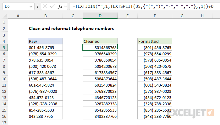
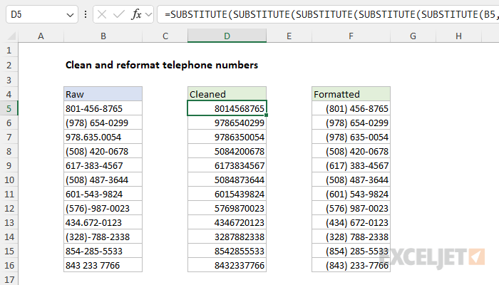
To clean up telephone numbers with inconsistent formatting, you can use a formula based on TEXTSPLIT and TEXTJOIN. In the worksheet shown, the formula in cell D5 is:
=TEXTJOIN("",1,TEXTSPLIT(B5,{"(",")","-"," ","."},,1))+0
As the formula is copied down, it removes spaces, dashes, periods, and parentheses and returns a single numeric value. In cell F5, Excel's built-in telephone Phone Number format has been applied to display the numbers in a format common in the US. Alternatively, you can concatenate values manually as explained below.
Note: TEXTSPLIT is only available in Excel 365. See below for an alternative formula that will work in older versions of Excel.
Generic formula
=TEXTJOIN("",1,TEXTSPLIT(A1,{"(",")","-"," ","."},,1))
Explanation
In this example, the goal is to clean up telephone numbers with inconsistent formatting and then reformat the numbers in the same way. In practice, this means we need to start by removing the extra non-numeric characters, including spaces, dashes, periods, and parentheses. Once these characters are removed, we can use Excel's number format system to format the numbers consistently. In the worksheet shown, the formula used to learn the numbers looks like this:
=TEXTJOIN("",1,TEXTSPLIT(B5,{"(",")","-"," ","."},,1))+0
Table of contents
- Removing extra characters
- Joining the numbers with punctuation
- Creating a single numeric value
- Applying number formatting with Format Cells
- Applying number formatting with the TEXT function
- All in one spill formula with the BYROW function
- Formula for older versions of Excel
- Line wrap trick for better readability
Removing extra characters
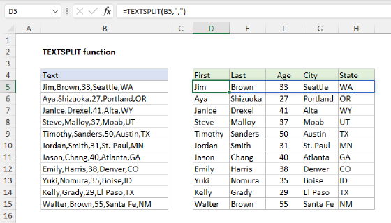
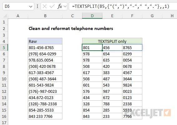
The first task is to remove the extra characters in the raw telephone numbers. These include the right and left parentheses "()", dashes or hyphens "-", space characters " ", and periods ".". The traditional approach to removing more than one value in an Excel formula is to nest together multiple SUBSTITUTE functions (see details below). However, since we have a limited number of characters to remove, a clever approach in this case is to use the TEXTSPLIT function like this:
TEXTSPLIT(B5,{"(",")","-"," ","."},,1)
Where the inputs to TEXTSPLIT are as follows:
- text - the text in cell B5
- col_delimiter - the array constant {"(",")","-"," ","."}
- row_delimiter - omitted
- ignore_empty - 1 (same as TRUE)
The key in this formula is the array constant with five values. Essentially, we are asking TEXTSPLIT to split the text at each parenthesis, dash, space, and period. We are also asking TEXTSPLIT to ignore any empty values that are generated. This is important because some of these delimiters have no actual value between them. The result is that the original telephone numbers are neatly split into three parts, and all five delimiters have been removed:
What's interesting about this (to me at least) is that when you use TEXTSPLIT to split text with different delimiters, the delimiters themselves are discarded in the process. This makes TEXTSPLIT an interesting way to remove multiple characters at the same time. The only drawback is that you have to combine the split text again, which is why we have TEXTJOIN in there as well. The CONCAT function would work equally well to join the numbers.
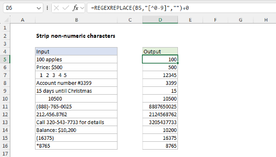
Note: if you have a lot of characters to remove, you can use a different formula to strip all non-numeric values at once, without calling out individual characters.
Joining the numbers with punctuation
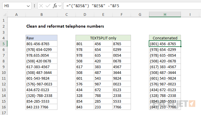
To create a final formatted result, one approach is to use manual concatenation to join the numbers together using the exact syntax you prefer. For example, in the screen below, the formula in cell H5 is:
="("&D5&") "&E5&" -"&F5
The key benefit of this approach is total control over the final result. You can insert specific characters with any logic you like. However, in the original worksheet shown above, we take a different approach: we create a single number, and then apply number formatting.
Creating a single numeric value
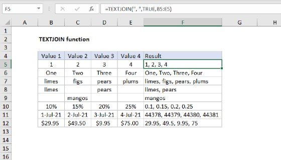
After the TEXTSPLIT splits the numbers and removes delimiters, the resulting array is returned to the TEXTJOIN function like this:
=TEXTJOIN("",1,{"801","456","8765"})+0
Because we have provided an empty string as the delimiter, the result from TEXTJOIN is a single text string like this:
="8014568765"+0
We then add zero to force Excel to convert the text value to the number 8014568765. Note: leading zeros will be removed when the value is converted to a number. If you need leading zeros, the simplest approach will be to concatenate manually as explained previously. There are pros and cons to both approaches.
Applying number formatting with Format Cells
The final step in this problem is to apply Excel's built-in telephone number format. To show this as a separate step, the worksheet below just pulls the value from column D into column F:
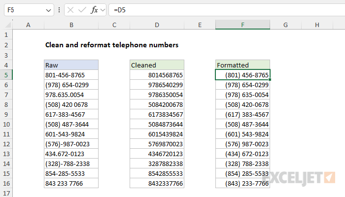
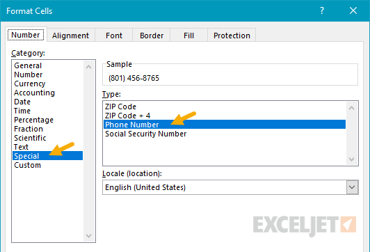
Next, select the range F5:F16 and use the keyboard shortcut Control + 1 to open the Format Cells window. Then apply the "Phone Number" format:
Applying number formatting with the TEXT function
Another good way to apply number formatting is to use the TEXT function with a custom number format like this:
TEXT(A1,"(000) 000-0000")
The result from TEXT will be a text string with the number in a format like (877) 437-8365.
All-in-one spill formula with the BYROW function
Matt Hanchett, a super smart subscriber to the Exceljet newsletter, emailed me to suggest this cool all-in-one dynamic array formula that will spill all cleaned and formatted numbers in one step:
=LET(
phoneList,B5:B16,
cleanList,BYROW(phoneList,LAMBDA(n,LET(chars,MID(n,SEQUENCE(LEN(n)),1),CONCAT(FILTER(chars,ISNUMBER(chars+0)))))),
validLen,IFERROR(LEN(cleanList),0)=10,
return,IF(validLen,TEXT(cleanList,"(000) 000-0000"),"Missing or invalid number."),
return
)
Unlike the original formula, which removes specific punctuation, this formula uses the FILTER function with the CONCAT function to strip all non-numeric characters. This code is packaged in a custom LAMBDA function called by the BYROW function, which iterates through all phone numbers one row at a time. It also features a nice error-checking step to confirm a 10-digit number and bail out with a friendly message when a number is not 10 digits. Note the definition of the "validLen" variable in the code above and how it is used in the next line.
Formula for older versions of Excel
Older versions of Excel do not provide the TEXTJOIN or TEXTSPLIT function, so we need a different formula. One traditional approach is to nest multiple SUBSTITUTE functions in a single formula like this:
=SUBSTITUTE(SUBSTITUTE(SUBSTITUTE(SUBSTITUTE(SUBSTITUTE(B5,"(",""),")",""),"-","")," ",""),".","")+0
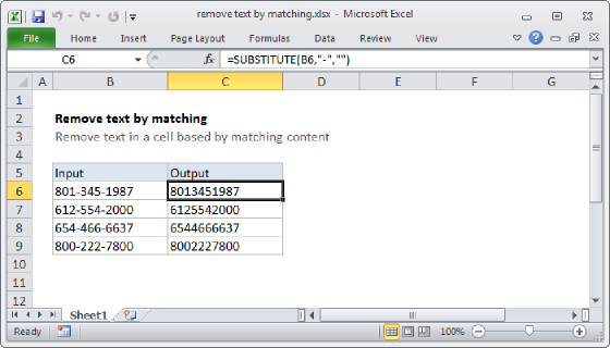
The formula runs from the inside out, with each SUBSTITUTE removing one character. The innermost SUBSTITUTE removes the left parentheses, and the result is handed to the next SUBSTITUTE, which removes the right parentheses, and so on. The workbook below shows the formula in action:
Whenever you use the SUBSTITUTE function, the result will be text. Because you can't apply a number format to text, we need to convert the text to a number. One way to do that is to add zero (+0), which automatically converts numbers in text format to numbers in numeric format. Finally, the "Special" telephone number format is applied to column D as explained above.
This page explains custom number formats with many examples.
Line wrap trick for better readability
When nesting multiple functions, it can be difficult to read the formula and keep all parentheses balanced. Excel doesn't care about extra white space in a formula, so you can add line breaks in the formula to make the formula more readable. For example, the formula above can be written as follows:
=
SUBSTITUTE(
SUBSTITUTE(
SUBSTITUTE(
SUBSTITUTE(
SUBSTITUTE(
A1,
"(",""),
")",""),
"-",""),
" ",""),
".","")
Note that the cell appears in the middle, with function names above and substitutions below. Not only does this make the formula easier to read, but it also makes it easier to add and remove substitutions. You can use this same trick to make nested IF statements easier to read as well.