=ROW([reference])- reference - [optional] A reference to a cell or range of cells.
Using the ROW function
The ROW function returns the row number for a cell or range. For example, =ROW(C3) returns 3, since C3 is the third row in the spreadsheet. When no reference is provided, ROW returns the row number of the cell which contains the formula. ROW takes just one argument, called reference, which can be empty, a cell reference, or a range. When no reference is provided, ROW returns the row number of the cell which contains the formula.
Examples
With a single cell reference, ROW returns the associated row number:
=ROW(A1) // returns 1
=ROW(E3) // returns 3
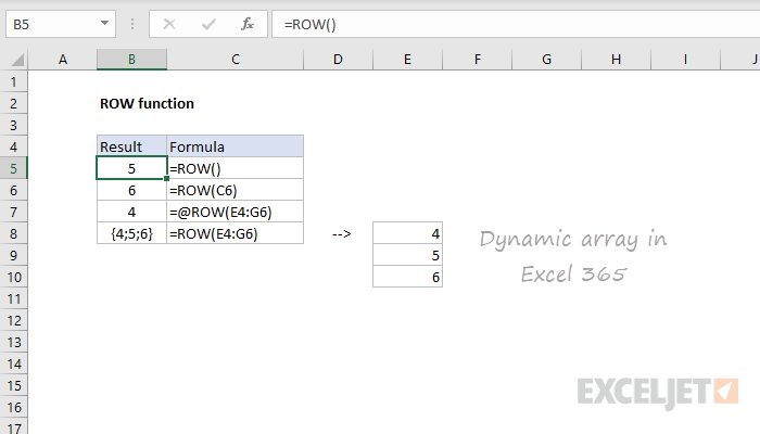
When a reference is not provided, ROW returns the row number of the cell the formula resides in. For example, if the following formula is entered in cell D6, the result is 6:
=ROW() // returns 6 in D6
When ROW is given a range, it returns the row numbers for that range:
=ROW(E4:G6) // returns {4,5,6}
In Excel 365, which supports dynamic array formulas, the result is an array {4,5,6} that spills vertically into three cells, starting with the cell that contains the formula. In earlier Excel versions, the first item of the array (4) will display in one cell only.
To get Excel 365 to return a single value, you can use the implicit intersection operator (@):
=@ROW(E4:G6) // returns 4
This @ symbol disables array behavior and tells Excel you want a single value.
Notes
- Reference can be a single cell address or a range of cells.
- Reference is optional and will default to the cell in which the ROW function exists.
- Reference cannot include multiple references or addresses.
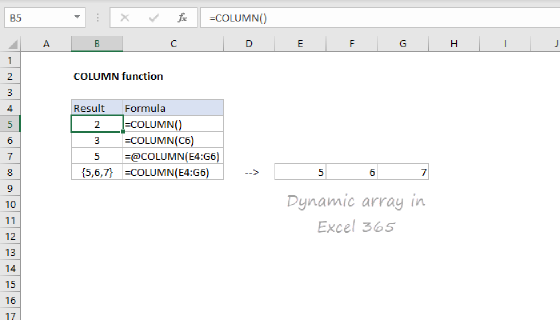
- To get column numbers, see the COLUMN function.
- To count rows, see the ROWS function.
- To lookup a row number, see the MATCH function.