Summary
Dynamic Arrays are the biggest change to Excel formulas in years. Maybe the biggest change ever. This is because Dynamic Arrays let you easily work with multiple values at the same time in a formula. This article provides an overview with many links and examples.
The key benefit of Dynamic Arrays is the ability to work with multiple values at the same time in a formula. This is a big upgrade and a welcome change. Dynamic Arrays solve some really hard problems in Excel, and will fundamentally change the way worksheets are designed. Once you see how they work, you'll never want to go back.
Availability
Dynamic arrays and the new functions below are only available Excel 365 and Excel 2021. Excel 2019 and earlier do not offer dynamic array formulas. For convenience, I'll use "Dynamic Excel" (Excel 365) and "Legacy Excel" (2019 or earlier) to differentiate the Excel versions below.
New functions
As part of the dynamic array update, Excel now includes 8 new functions that directly leverage dynamic arrays to solve problems that are traditionally hard to solve with conventional formulas. Click the links below for details and examples for each function:
| Function | Purpose |
|---|---|
| FILTER | Filter data and return matching records |
| RANDARRAY | Generate an array of random numbers |
| SEQUENCE | Generate an array of sequential numbers |
| SORT | Sort range by column |
| SORTBY | Sort range by another range or array |
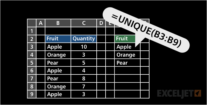
| UNIQUE | Extract unique values from a list or range |
| XLOOKUP | Modern replacement for VLOOKUP |
| XMATCH | Modern replacement for the MATCH function |
Video: New dynamic array functions in Excel (about 3 minutes).
As of September 2024, almost 50 new functions have been added to Excel!
Example
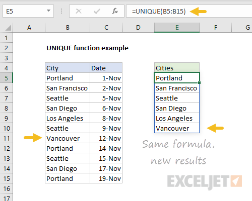
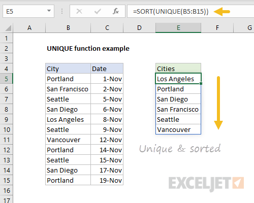
Before we get into the details, let's look at a simple example. Below we are using the new UNIQUE function to extract unique values from the range B5:B15, with a single formula entered in E5:
=UNIQUE(B5:B15) // return unique values in B5:B15
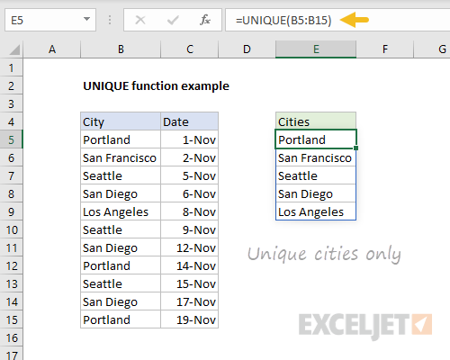
The result is a list of the five unique city names, which appear in E5:E9.
Like all formulas, UNIQUE will update automatically when data changes. Below, Vancouver has replaced Portland on row 11. The result from UNIQUE now includes Vancouver:
Spilling - one formula, many values
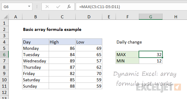
In Dynamic Excel, formulas that return multiple values will "spill" these values directly onto the worksheet. This will immediately be more logical to formula users. It is also a fully dynamic behavior – when source data changes, spilled results will immediately update.
The rectangle that encloses the values is called the "spill range". You will notice that the spill range has special highlighting. In the UNIQUE example above, the spill range is E5:E10.
When data changes, the spill range will expand or contract as needed. You might see new values added, or existing values disappear. In this way, a spill range is a new kind of dynamic range.
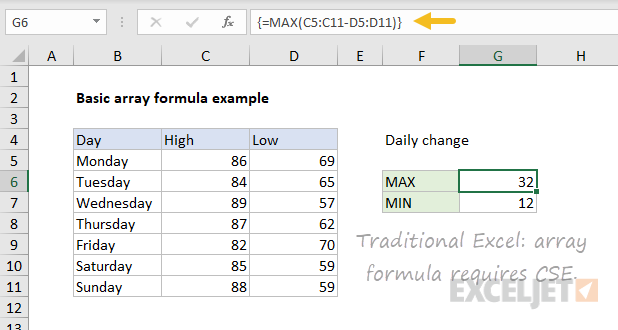
In Legacy Excel, by contrast, you can see multiple results returned by an array formula in the formula bar if you use F9 to inspect the formula. However, unless the formula is entered as a multi-cell array formula, only one value will be displayed on the worksheet. This behavior has always made array formulas difficult to understand. Spilling makes array formulas more intuitive.
Note: when spilling is blocked by other data, you'll see a #SPILL error. Once you make room for the spill range, the formula will automatically spill.
Video: Spilling and the spill range
Spill range reference
To refer to a spill range, use a hash symbol (#) after the first cell in the range. For example, to reference the results from the UNIQUE function above use:
=E5# // reference UNIQUE results
This is the same as referencing the entire spill range, and you'll see this syntax when you write a formula that refers to a complete spill range.
You can feed a spill range reference into other formulas directly. For example, to count the number of cities returned by UNIQUE, you can use:
=COUNTA(E5#) // count unique cities
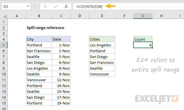
When the spill range changes, the formula will reflect the latest data.
Massive simplification
The addition of new dynamic array formulas means certain formulas can be drastically simplified. Here are a few examples:
- Extract and list unique values (before | after)
- Count unique values (before | after)
- Filter and extract records (before | after)
- Extract partial matches (before | after)
The power of one
One of the most powerful benefits of the "one formula, many values" approach is less reliance on absolute or mixed references. As a dynamic array formula spills results onto the worksheet, references remain unchanged, but the formula generates correct results.
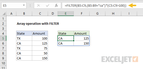
For example, below we use the FILTER function to extract records in group "A". In cell F5, a single formula is entered:
=FILTER(B5:D11,B5:B11="a") // references are relative
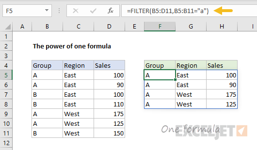
Notice both ranges are unlocked relative references, but the formula works perfectly.
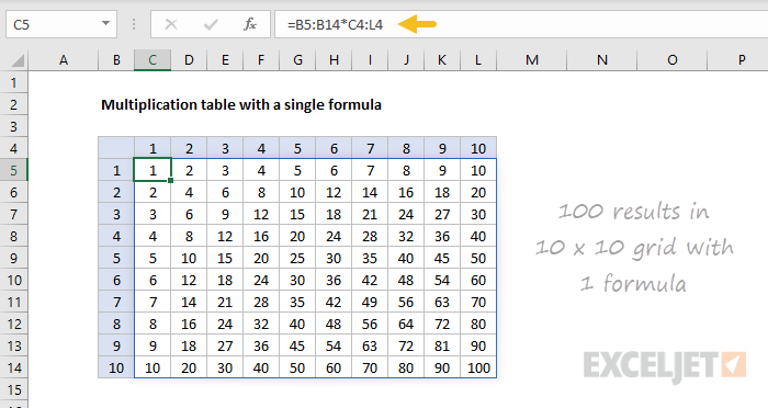
This is a huge benefit for many users because it makes the process of writing formulas so much simpler. For another good example, see the multiplication table below.
Chaining functions
Things get really interesting when you chain together more than one dynamic array function. Perhaps you want to sort the results returned by UNIQUE? Easy. Just wrap the SORT function around the UNIQUE function like this:
As before, when source data changes, new unique results automatically appear, nicely sorted.
Native behavior
It's important to understand that dynamic array behavior is native and deeply integrated. When any formula returns multiple results, these results will spill into multiple cells on the worksheet. This includes older functions not originally designed to work with dynamic arrays.
For example, in Legacy Excel, if we give the LEN function a range of text values, we'll see a single result. In Dynamic Excel, if we give the LEN function a range of values, we'll see multiple results. This screen below shows the old behavior on the left and the new behavior on the right:
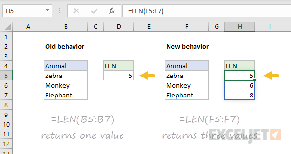
This is a huge change that can affect all kinds of formulas. For instance, the VLOOKUP function is designed to fetch a single value from a table, using a column index. However, in Dynamic Excel, if we give VLOOKUP more than one column index using an array constant like this:
=VLOOKUP("jose",F7:H10,{1,2,3},0)
VLOOKUP will return multiple columns:
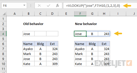
In other words, even though VLOOKUP was never designed to return multiple values, it can now do so, thanks to the new formula engine in Dynamic Excel.
All formulas
Finally, note that dynamic arrays work with all formulas not just functions. In the example below cell C5 contains a single formula:
=B5:B14*C4:L4
The result spills into a 10 by 10 range that includes 100 cells:
If the numbers in the ranges B5:B14 and C4:L4 where are themselves dynamic arrays (i.e. created with the SEQUENCE function), the spill reference operator can be used like this:
=B5#*C4# // returns same 10 x 10 array
Arrays go mainstream
With the rollout of dynamic arrays, the word "array" is going to pop up much more often. In fact, you may see "array" and "range" used almost interchangeably. You'll see arrays in Excel enclosed in curly braces like this:
{1,2,3} // horizontal array
{1;2;3} // vertical array
Array is a programming term that refers to a list of items that appear in a particular order. The reason arrays come up so often in Excel formulas is that arrays can perfectly express the values in a range of cells.
Video: What is an array?
Array operations become important
Because Dynamic Excel formulas can easily work with multiple values, array operations will become more important. The term "array operation" refers to an expression that runs a logical test or math operation on an array. For example, the expression below tests if values in B5:B9 are equal to "ca"
=B5:B9="ca" // state = "ca"
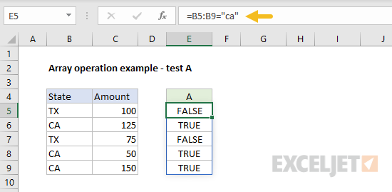
because there are 5 cells in B5:B9, the result is 5 TRUE/FALSE values in an array:
{FALSE;TRUE;FALSE;TRUE;TRUE}
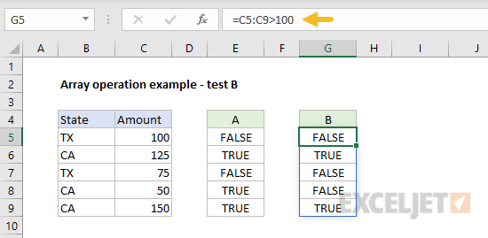
The array operation below checks for amounts greater than 100:
=C5:C9>100 // amounts > 100
The final array operation combines test A and test B in a single expression:
=(B5:B9="ca")*(C5:C9>100) // state = "ca" and amount > 100
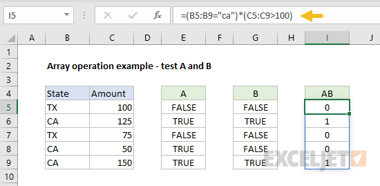
Note: Excel automatically coerces the TRUE and FALSE values to 1 and 0 during the math operation.
To bring this back to dynamic array formulas in Excel, the example below demonstrates how we can use exactly the same array operation inside the FILTER function as the include argument:
FILTER returns the two records where state = "ca" and amount > 100.
For a demonstration, see: How to filter with two criteria (video).
New and old array formulas
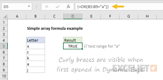
In Dynamic Excel, there is no need to enter array formulas with control + shift + enter. When a formula is created, Excel checks if the formula might return multiple values. If so, it will automatically be saved as a dynamic array formula, but you will not see curly braces. The example below shows a typical array formula entered in Dynamic Excel:
If you open the same formula in Legacy Excel, you'll see curly braces:
Going the other direction, when a "traditional" array formula is opened in Dynamic Excel, you will see the curly braces in the formula bar. For example, the screen below shows a simple array formula in Legacy Excel:
However, if you re-enter the formula with no changes, the curly braces are removed, and the formula returns the same result:

The bottom line is that array formulas entered with control + shift + enter (CSE) still work to maintain compatibility, but you shouldn't need to enter array formulas with CSE in Dynamic Excel.
Spilling limitations and the plus (+) operator
The term "lifting" refers to an array calculation behavior in Excel formulas. When you give a range or array to a function not programmed to accept arrays natively (i.e. an older function), Excel will "lift" the function and call it multiple times, one time for each value in the array. The result is an array with the same dimensions as the input array. Lifting is a built-in behavior that happens automatically.
In Dynamic Excel, some older functions like EOMONTH "resist" spilling when provided a range. So, for example, EOMONTH(A1:A5,1) will return #VALUE even with valid dates in A1:A5. This limitation comes from certain functions expecting a single value instead of a range. The #VALUE! error is essentially reporting the range as an unexpected value. However, adding an operator in front of the reference will often fix the problem. For example, EOMONTH(+A1:A5,1) will work and spill properly. This is because adding the + in front of A1:A5 forces Excel to evaluate the expression first, before the function runs. The result of +A1:A5 is an array containing 5 values, which are then passed into EOMONTH as the start date. EOMONTH returns 5 results through the normal process of lifting, which is not function-specific. Other functions that have this same limitation include EDATE, ISEVEN, ISODD, YEARFRAC, WORKDAY, and WORKDAY.INTL.
For more details and a list of functions that have this problem, see: Why some functions won't spill.
The @ character
With the introduction of dynamic arrays, you're going to see the @ character appear more often in formulas. The @ character enables a behavior known as "implicit intersection". Implicit intersection is a logical process where many values are reduced to one value.
In Legacy Excel, implicit intersection is a silent behavior used (when necessary) to reduce multiple values to a single result in one cell. In Dynamic Excel, it is not typically needed, since multiple results can spill onto the worksheet. When it is needed, implicit intersection is invoked manually with the @ character.
When opening spreadsheets created in an older version of Excel, you may see the @ character added automatically to existing formulas that have the potential to return many values. In Legacy Excel, a formula that returns multiple values won't spill on the worksheet. The @ character forces this same behavior in Dynamic Excel so that the formula behaves the same way and returns the same result as it did in the original Excel version.
In other words, the @ is added to prevent an older formula from spilling multiple results onto the worksheet. Depending on the formula, you may be able to remove the @ character and the behavior of the formula will not change.
Summary
- Dynamic Arrays will make certain formulas much easier to write.
- You can now filter matching data, sort, and extract unique values easily with formulas.
- Dynamic Array formulas can be chained (nested) to do things like filter and sort.
- Formulas that return more than one value will automatically spill.
- It is not necessary to use Ctrl+Shift+Enter to enter an array formula.
- Dynamic array formulas are only available in Excel 365.


