Summary
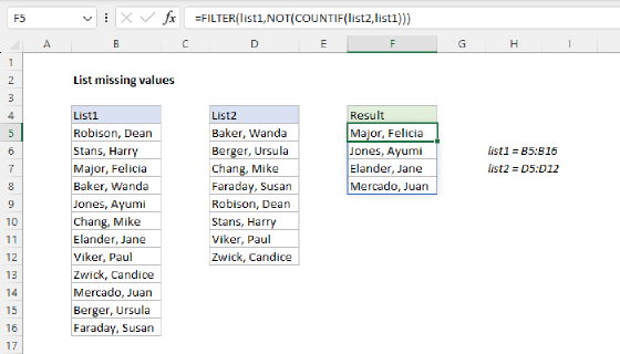
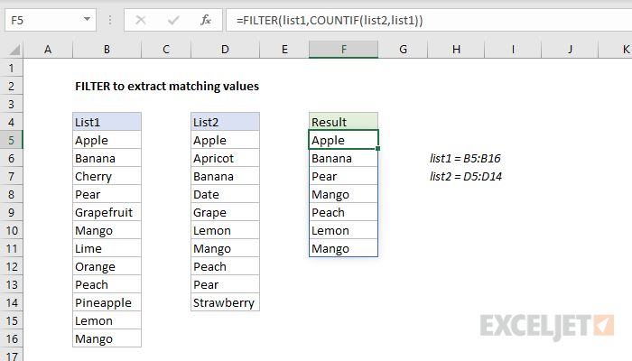
To filter data to extract matching values in two lists, you can use the FILTER function and the COUNTIF or COUNTIFS function. In the example shown, the formula in F5 is:
=FILTER(list1,COUNTIF(list2,list1))
where list1 (B5:B16) and list2 (D5:D14) are named ranges. The result returned by FILTER includes only the values in list1 that appear in list2.
Note: FILTER is a new dynamic array function in Excel 365.
Generic formula
=FILTER(list1,COUNTIF(list2,list1))
Explanation
This formula relies on the FILTER function to retrieve data based on a logical test built with the COUNTIF function:
=FILTER(list1,COUNTIF(list2,list1))
working from the inside out, the COUNTIF function is used to create the actual filter:
COUNTIF(list2,list1)
Notice we are using list2 as the range argument, and list1 as the criteria argument. In other words, we are asking COUNTIF to count all values in list1 that appear in list2. Because we are giving COUNTIF multiple values for criteria, we get back an array with multiple results:
{1;1;0;1;0;1;0;0;1;0;1;1}
Note the array contains 12 counts, one for each value in list1. A zero value indicates a value in list1 that is not found in list2. Any other positive number indicates a value in list1 that is found in list2. This array is returned directly to the FILTER function as the include argument:
=FILTER(list1,{1;1;0;1;0;1;0;0;1;0;1;1})
The FILTER function uses the array as a filter. Any value in list1 associated with a zero is removed, while any value associated with a positive number survives.
The result is an array of 7 matching values which spill into the range F5:F11. If data changes, FILTER will recalculate and return a new list of matching values based on the new data.
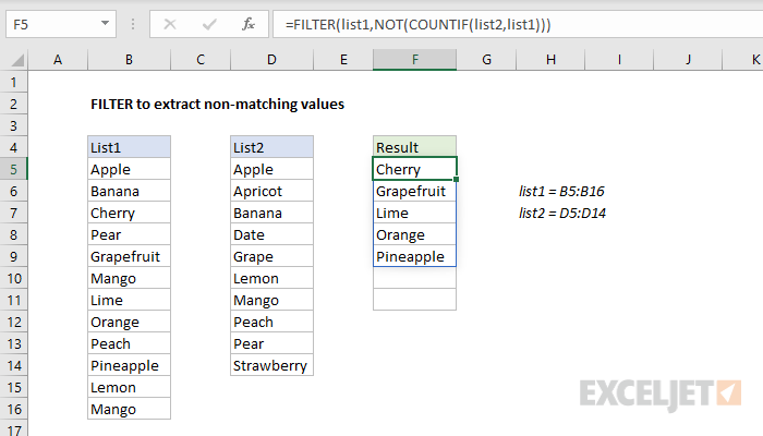
Non-matching values
To extract non-matching values from list1 (i.e. values in list1 that don't appear in list2) you can add the NOT function to the formula like this:
=FILTER(list1,NOT(COUNTIF(list2,list1)))
The NOT function effectively reverses the result from COUNTIF – any non-zero number becomes FALSE, and any zero value becomes TRUE. The result is a list of the values in list1 that are not present in list2.
With INDEX
It is possible to create a formula to extract matching values without the FILTER function, but the formula is more complex. One option is to use the INDEX function in a formula like this:
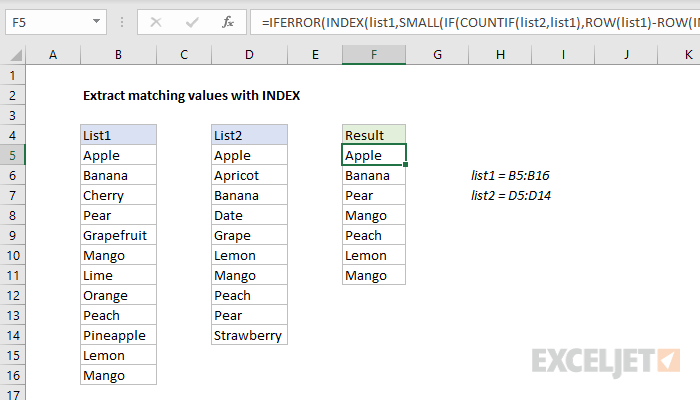
The formula in G5, copied down is:
=IFERROR(INDEX(list1,SMALL(IF(COUNTIF(list2,list1),ROW(list1)-ROW(INDEX(list1,1,1))+1),ROWS($F$5:F5))),"")
Note: this is an array formula and must be entered with control + shift + enter, except in Excel 365.
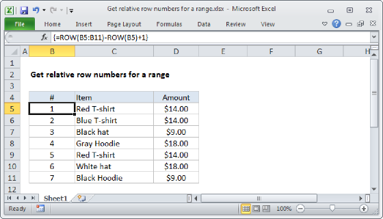
The core of this formula is the INDEX function, which receives list1 as the array argument. Most of the remaining formula simply calculates the row number to use for matching values. This expression generates a list of relative row numbers:
ROW(list1)-ROW(INDEX(list1,1,1))+1
which returns an array of 12 numbers representing the rows in list1:
{1;2;3;4;5;6;7;8;9;10;11;12}
These are filtered with the IF function and the same logic used above in FILTER, based on the COUNTIF function:
COUNTIF(list2,list1) // find matching values
The resulting array looks like this:
{1;2;FALSE;4;FALSE;6;FALSE;FALSE;9;FALSE;11;12} // result from IF
This array is delivered directly to the SMALL function, which is used to fetch the next matching row number as the formula is copied down the column. The k value for SMALL (think nth) is calculated with an expanding range:
ROWS($G$5:G5) // incrementing value for k
The IFERROR function is used to trap errors that occur when the formula is copied down and runs out of matching values. For another example of this idea, see this formula.