Gantt chart

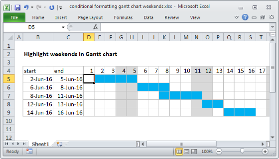
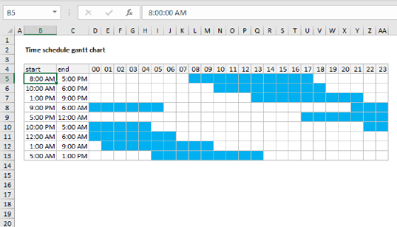
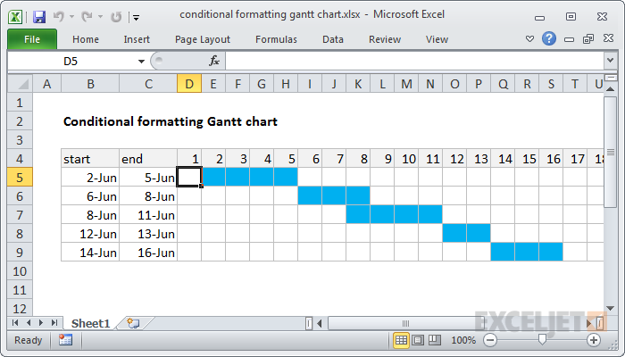
To build a Gantt chart, you can use Conditional Formatting with a formula based on the AND function. In the example shown, the formula applied to D5 is:

=AND(D$4>=$B5,D$4<=$C5)

Explanation

The trick with this approach is the calendar header (row 4), which is just a series of valid dates, formatted with the custom number format "d". With a static date in D4, you can use =D4+1 to populate the calendar. This makes it easy to set up a conditional formatting rule that compares the date associated with each column with the dates in columns B and C.

The formula is based on the AND function, configured with two conditions. The first conditions checks to see if the column date is greater than or equal to the start date:

D$4>=$B5

The second condition checks that the column date is less than or equal to the end date:

D$4<=$C5

When both conditions return true, the formula returns TRUE, triggering the blue fill for the cells in the calendar grid.

Note: both conditions use mixed references to ensure that the references update correctly as conditional formatting is applied to the calendar grid.