Find duplicate values in two columns

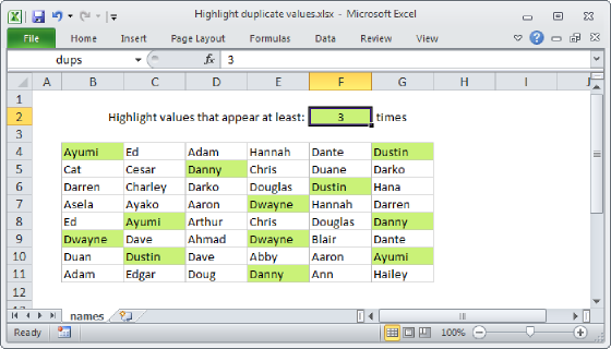
To highlight duplicate values in two or more columns, you can use conditional formatting with on a formula based on the COUNTIF and AND functions.

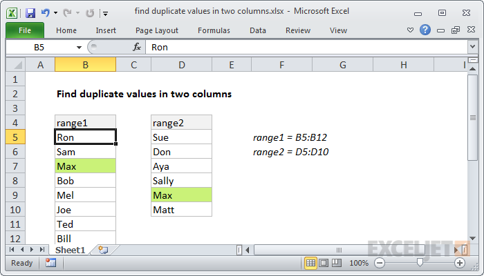
In the example shown, the formula used to highlight duplicate values is:

=AND(COUNTIF(range1,B5),COUNTIF(range2,B5))

Both ranges were selected at the same when the rule was created.

Explanation

This formula uses two named ranges, "range1" (B5:B12) and "range2" (D5:D10).

The core of this formula is the COUNTIF function, which returns a count of each value in both range inside the AND function:

COUNTIF(range1,B5) // count in range1
COUNTIF(range2,B5) // count in range2

COUNTIF will either return zero (evaluated as FALSE) or a positive number (evaluated as TRUE) for each value in both ranges.

If both counts are positive (i.e. non-zero), the AND function will return TRUE and trigger the conditional format.