LOOKUP Function

Use the LOOKUP function to look up a value in a one-column or one-row range, and retrieve a value from the same position in another one-column or one-row range. The lookup function has two forms, vector and array. The majority of this article describes the vector form, but the last example below illustrates the array form.

The LOOKUP function accepts three arguments: lookup_value, lookup_vector, and result_vector. The first argument, lookup_value, is the value to look for. The second argument, lookup_vector, is a one-row, or one-column range to search. LOOKUP assumes that lookup_vector is sorted in ascending order. The third argument, result_vector, is a one-row, or one-column range of results. Result_vector is optional. When result_vector is provided, LOOKUP locates a match in the lookup_vector, and returns the corresponding value from result_vector. If result_vector is not provided, LOOKUP returns the value of the match found in lookup_vector.

LOOKUP has default behaviors that make it useful when solving certain problems. For example, LOOKUP can be used to retrieve an approximate-matched value instead of a position and to find the last value in a row or column. LOOKUP assumes that values in lookup_vector are sorted in ascending order and always performs an approximate match. When LOOKUP can't find a match, it will match the next smallest value.

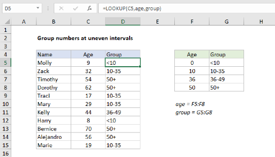
Example #1 - basic usage

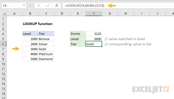
In the example shown above, the formula in cell F5 returns the value of the match found in column B. Note that result_vector is not provided:

=LOOKUP(F4,B5:B9) // returns match in level

The formula in cell F6 returns the corresponding Tier value from column C. Notice in this case, both lookup_vector and result_vector are provided:

=LOOKUP(F4,B5:B9,C5:C9) // returns corresponding tier 

In both formulas, LOOKUP automatically performs an approximate match and it is therefore important that lookup_vector is sorted in ascending order.

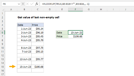
Example #2 - last non-empty cell

LOOKUP can be used to get the value of the last filled (non-empty) cell in a column. In the screen below, the formula in F6 is:

=LOOKUP(2,1/(B:B<>""),B:B)

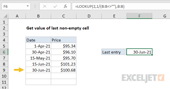
Note the use of a full column reference. This is not an intuitive formula, but it works well. The key to understanding this formula is to recognize that the lookup_value of 2 is deliberately larger than any values that will appear in the lookup_vector. Detailed explanation here.

Example #3 - latest price

Similar to the above example, the lookup function can be used to look up the latest price in data sorted in ascending order by date. In the screen below, the formula in G5 is:

=LOOKUP(2,1/(item=F5),price)

where item (B5:B12) and price (D5:D12) are named ranges. 

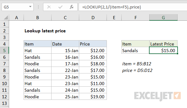
When lookup_value is greater than all values in lookup_array, default behavior is to "fall back" to the previous value. This formula exploits this behavior by creating an array that contains only 1s and errors, then deliberately looking for the value 2, which will never be found. More details here.

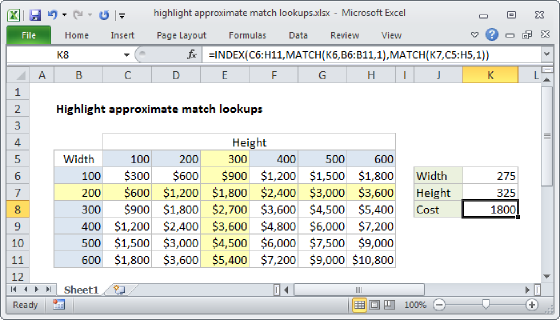
Example #4 - array form

The LOOKUP function has an array form as well. In the array configuration, LOOKUP takes just two arguments: the lookup_value, and a single two-dimensional array:

LOOKUP(lookup_value, array) // array form

In the array form, LOOKUP evaluates the array and automatically changes behavior based on the array dimensions. If the array is wider than tall, LOOKUP looks for the lookup value in the first row of the array (like HLOOKUP). If the array is taller than wide (or square), LOOKUP looks for the lookup value in the first column (like VLOOKUP). In either case, LOOKUP returns a value at the same position from the last row or column in the array. The example below shows how the array form works. The formula in F5 is configured to use a vertical array and the formula in F6 is configured to use a horizontal array:

=LOOKUP(E5,B5:C9) // vertical array
=LOOKUP(E6,C11:G12) // horizontal array

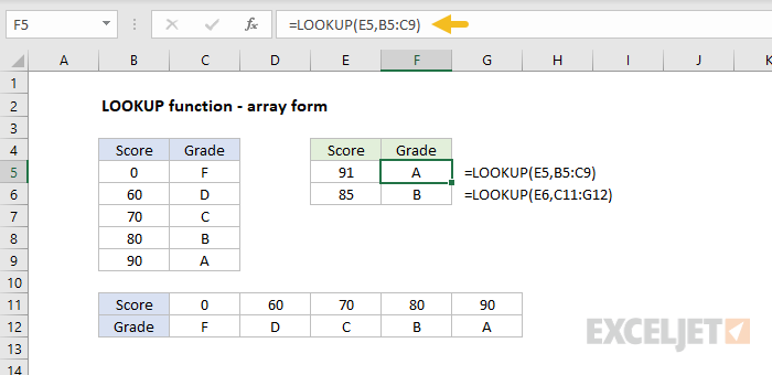
The vertical and horizontal arrays contain the same values; only the orientation is different.

Note: Microsoft discourages the use of the array form and suggests VLOOKUP and HLOOKUP as better options.

Notes

• LOOKUP assumes that lookup_vector is sorted in ascending order.
• When lookup_value can't be found, LOOKUP will match the next smallest value.
• When lookup_value is greater than all values in lookup_vector, LOOKUP matches the last value.
• When lookup_value is less than the first value in lookup_vector, LOOKUP returns #N/A.
• Result_vector must be the same size as lookup_vector.
• LOOKUP is not case-sensitive