Get last entry by month and year

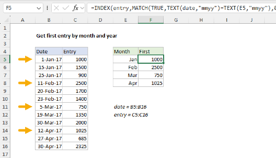
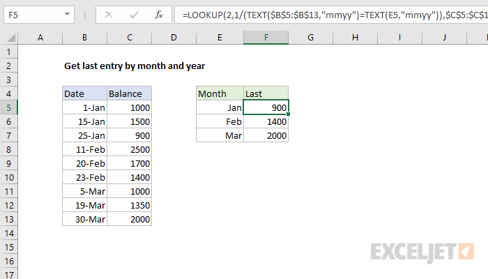
To lookup the last entry in a table by month and year, you can use the LOOKUP function with the TEXT function. In the example shown, the formula in F5 is:

=LOOKUP(2,1/(TEXT($B$5:$B$13,"mmyy")=TEXT(E5,"mmyy")),$C$5:$C$13)

where B5:B13 and E5:E7 contain valid dates, and C5:C13 contains amounts.

Explanation

Note: the lookup_value of 2 is deliberately larger than any values in the lookup_vector, following the concept of bignum.

Working from the inside out, the expression:

(TEXT($B$5:$B$13,"mmyy")=TEXT(E5,"mmyy"))

generates strings like "0117" using the values in column B and E, which are then compared to each other. The result is an array like this:

{TRUE;TRUE;TRUE;FALSE;FALSE;FALSE;FALSE;FALSE;FALSE}

where TRUE represents dates in the same month and year. The number 1 is then divided by this array. The result is an array of either 1's or divide by zero errors (#DIV/0!):

{1;1;1;#DIV/0!;#DIV/0!;#DIV/0!;#DIV/0!;#DIV/0!;#DIV/0!}

which goes into LOOKUP as the lookup array. LOOKUP assumes data is sorted in ascending order and always does an approximate match. When the lookup value of 2 can't be found, LOOKUP will match the previous value, so lookup will match the last 1 in the array.

Finally, LOOKUP returns the corresponding value in result_vector, which contains the amounts in C5:C13.