Summary
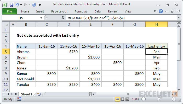
To retrieve a date associated with a last entry tabular data, you can use a formula based on the LOOKUP function. In the example shown the formula in H5 is:
=LOOKUP(2,1/(C5:G5<>""),C$4:G$4)
Generic formula
=LOOKUP(2,1/(row<>""),header)
Explanation
Working from the inside out, the expression C5:G5<>"" returns an array of true and false values:
{FALSE,TRUE,FALSE,FALSE,FALSE}
The number 1 is divided by this array, which creates a new array composed of either 1's or #DIV/0! errors:
{#DIV/0!,1,#DIV/0!,#DIV/0!,#DIV/0!}
This array is used as the lookup_vector.
The lookup_value is 2, but the largest value in the lookup_array is 1, so LOOKUP will match the last 1 in the array.
Finally, LOOKUP returns the corresponding value in result_vector, from the dates in the range C$4:G$4.
Note: the result in column H is a date from row 5, formatted with the custom format "mmm" to show an abbreviated month name only.
Zeros instead of blanks
You might have a table with zeros instead of blank cells:
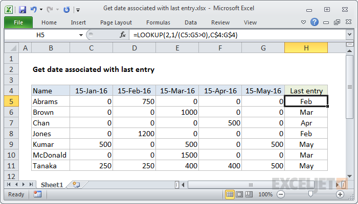
In that case, you can adjust the formula to match values greater than zero like so:
=LOOKUP(2,1/(C5:G5>0),C$4:G$4)
Multiple criteria
You can extend criteria by adding expressions to the denominator with boolean logic. For example, to match the last value greater than 400, you can use a formula like this:
=LOOKUP(2,1/((C5:G5<>"")*(C5:G5>400)),C$4:G$4)