Summary
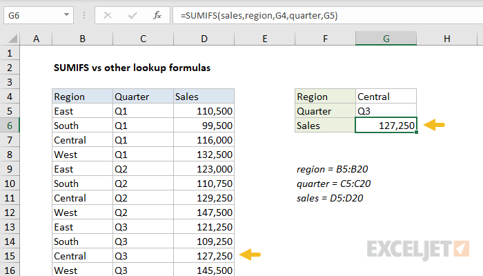
In certain cases, you can use SUMIFS like a lookup formula to retrieve a numeric value. In the example shown, the formula in G6 is:
=SUMIFS(sales,region,G4,quarter,G5)
where region (B5:B20), quarter (C5:C20), and sales (D5:D20) are named ranges.
The result is Q3 sales for the Central region, 127,250.
Explanation
If you are new to the SUMIFS function, you can find a basic overview with many examples here.
The SUMIFS function is designed to sum numeric values based on one or more criteria. In specific cases however, you may be able to use SUMIFS to "look up" a numeric value that meets required criteria. The main reasons to do this are simplicity and speed.
In the example shown, we have quarterly sales data for four regions. We start off by giving SUMIFS a sum range, and the first condition, which tests region for the value in G4, "Central":
=SUMIFS(sales,region,G4 // sum range, region is "Central"
- Sum range is sales (D5:D20)
- Criteria range 1 is region (B5:B20)
- Criteria 1 is G4 ("Central")
We then add the second range/criteria pair, which checks quarter:
=SUMIFS(sales,region,G4,quarter,G5) // and quarter is "Q3"
- Criteria range 2 is quarter (C5:C20)
- Criteria 2 is G5 ("Q3")
With these criteria, SUMIFS returns 127,250, the Central Q3 sales number.
The behavior of SUMIFS is to sum all matching values. However, because there is just one matching value, the result is the same as the value itself.
Below, we look at several lookup formula options.
Lookup formula options
This section briefly reviews other formula options that yield the same result. With the exception of SUMPRODUCT (at the bottom), these are more traditional lookup formulas that locate the position of the target value, and return the value at that location.
With VLOOKUP
Unfortunately, VLOOKUP is not a good solution to this problem. With a helper column, it is possible to build a VLOOKUP formula to match with multiple criteria (example here), but it's an awkward process that requires you to tinker with the source data.
With INDEX and MATCH
INDEX and MATCH is a very flexible lookup combination that can be used for all kinds of lookup problems, and this example is no exception. With INDEX and MATCH, we can lookup sales by region and quarter with an array formula like this:
{=INDEX(sales,MATCH(1,(region=G4)*(quarter=G5),0))}
Note: this is an array formula, and must be entered with control + shift + enter.
The trick with this approach is to use boolean logic with array operations inside the MATCH function to build an array of 1s and 0s as the lookup array. Then we can ask the MATCH function find the number 1. Once the lookup array is created, the formula resolves to:
=INDEX(sales,MATCH(1,{0;0;0;0;0;0;0;0;0;0;1;0;0;0;0;0},0))
With only 1 remaining in the lookup array, MATCH returns a position of 11 to the INDEX function, and INDEX returns the sales number at that position, 127,250.
For more details, see : INDEX and MATCH with multiple criteria
With XLOOKUP
XLOOKUP is a flexible new function in Excel that can handle arrays natively. With XLOOKUP, we can use exactly the same approach as with INDEX and MATCH, using boolean logic and array operations to create a lookup array:
=XLOOKUP(1,(region=G4)*(quarter=G5),sales)
Once the array operations have run, the formula resolves to:
=XLOOKUP(1,{0;0;0;0;0;0;0;0;0;0;1;0;0;0;0;0},sales)
And XLOOKUP returns the same result as above, 127,250.
More: XLOOKUP with multiple criteria
Dynamic Array Formulas are available in Office 365 only.
With LOOKUP
The LOOKUP function is an older function in Excel that many people don't even know about. One of LOOKUP's key strengths is that it can handle arrays natively. However, LOOKUP has a few distinct weaknesses:
- Can't be locked in "exact match mode"
- Always assumes lookup data is sorted, A-Z
- Always returns an approximate match (if exact match can't be found)
Nonetheless, LOOKUP can be used to solve this problem nicely like this:
=LOOKUP(2,1/((region=G4)*(quarter=G5)),sales)
which simplifies to:
=LOOKUP(2,{#DIV/0!;#DIV/0!;#DIV/0!;#DIV/0!;#DIV/0!;#DIV/0!;#DIV/0!;#DIV/0!;#DIV/0!;#DIV/0!;1;#DIV/0!;#DIV/0!;#DIV/0!;#DIV/0!;#DIV/0!},sales)
If you look closely, you can see a single number 1 in a sea of #DIV/0! errors. This represents the value we want to retrieve.
We use a lookup value of 2 because we can't guarantee the array is sorted. So, we force all non-matching rows to errors, and ask LOOKUP to find a 2. LOOKUP ignores the errors and dutifully scans the entire array looking for 2. When the number 2 can't be found, LOOKUP "backs up" and matches the last non-error value, which is the 1 in the 11th position. The result is the same as above, 127,250.
More detailed explanation here.
With SUMPRODUCT
As usual, you can also use the Swiss Army Knife SUMPRODUCT function to solve this problem as well. The trick is to use boolean logic and array operations to "zero out" all but the one value we want:
=SUMPRODUCT(sales*((region=G4)*(quarter=G5)))
After the array math inside SUMPRODUCT is complete, the formula simplifies to:
=SUMPRODUCT({0;0;0;0;0;0;0;0;0;0;127250;0;0;0;0;0})
This is technically not really a lookup formula, but it behaves like one. With just a single array to process, the SUMPRODUCT function returns the sum of the array, 12,7250.
See this example for a more complete explanation.
In spirit, the SUMPRODUCT option is closest to the SUMIFS formula since we are summing values based on multiple criteria. As before, it works fine as long as there is only one matching result.
Summary
SUMIF can indeed be used like a lookup formula, and configuration may be simpler than a more conventional lookup formula. In addition, if you are working with a large data set, SUMIFS will be a very fast option. However, you must keep in mind two key requirements:
- The result must be numeric data
- Criteria must match only one result
If the situation doesn't meet both requirements, SUMIFS is not a good choice.