
Purpose
Return value
Syntax
=IFERROR(value,value_if_error)- value - The value, reference, or formula to check for an error.
- value_if_error - The value to return if an error is found.
Using the IFERROR function
The IFERROR function returns a custom result when a formula returns an error and a normal result when a formula calculates without an error. The typical syntax for the IFERROR function looks like this:
=IFERROR(formula,custom)
In the example above, "formula" represents a formula that might return an error, and "custom" represents the value that should be returned if the formula returns an error. This makes IFERROR an elegant way to trap and manage errors in one step. Before the introduction of IFERROR, it was necessary to use more complicated nested IF statements together with the older ISERROR function.
You can use the IFERROR function to trap and handle errors produced by other formulas or functions. IFERROR checks for the following errors: #N/A, #VALUE!, #REF!, #DIV/0!, #NUM!, #NAME?, or #NULL!.
Example 1 - Trap #DIV/0! errors
In the example shown, the formula in E5 copied down is:
=IFERROR(C5/D5,0)
This formula catches the #DIV/0! error that occurs when the quantity field is empty or zero, and replaces it with zero. You are free to change the zero (0) to suit your needs. For example, to display nothing, you could use an empty string ("") instead of zero:
=IFERROR(C5/D5,"")
This version of the formula will trap the #DIV/0! error and return an empty string, which looks like an blank cell.
Example 2 - request input before calculating
Sometimes you may want to suppress a calculation until the worksheet receives specific input. For example, if A1 contains 10, B1 is blank, and C1 contains the formula =A1/B1, the following formula will return a #DIV/0 error if B1 is empty:
=IFERROR(A1/B1) // returns #DIV! if B1 is empty
The formula below has been modified to use the IFERROR function to trap the #DIV/0! error and remap it to the message "Please enter a value in B1".
=IFERROR(A1/B1,"Please enter a value in B1")
As long as B1 is empty, C1 will display the message "Please enter a value in B1" if B1. When a number is entered in B1, the formula will return the result of A1/B1.
Example 3 - Sum and ignore errors
A common problem in Excel is that errors in data will corrupt the results of other formulas. For example, in the worksheet shown below, the goal is to sum values in the range D5:D15. However, because the range D5:D15 contains #N/A errors, the SUM function will return #N/A:
=SUM(D5:D15) // returns #N/A

To ignore the #N/A errors and sum the remaining values, we can adjust the formula to use the IFERROR function like this:
=SUM(IFERROR(D5:D15,0)) // returns 152.50
Essentially, we use IFERROR to map the errors to zero and then sum the result. For more details and alternatives, see Sum and ignore errors.
Example 3 - VLOOKUP #N/A
When VLOOKUP cannot find a lookup value, it returns an #N/A error. You can use the IFERROR function to catch the #N/A error VLOOKUP throws when a lookup value isn't found like this:
=IFERROR(VLOOKUP(value,data,column,0),"Not found")
In this example, the IFERROR function evaluates the result returned by VLOOKUP. If no error is present, the result is returned normally. However, if VLOOKUP returns an #N/A error, IFERROR catches the error and returns "Not Found".
IFERROR or IFNA?
The IFERROR function is useful, but it is a rather blunt instrument that will trap all kinds of errors. For example, if a function is misspelled in a formula, Excel will return the #NAME? error and IFERROR will catch that error too, and return an alternate result. This can cause IFERROR to hide an important problem. In most cases, it makes more sense to use the IFNA function with VLOOKUP instead of IFERROR.
=IFNA(VLOOKUP(value,data,column,0),"Not found")
Unlike IFERROR, IFNA only traps the #N/A error.
Other error functions
Excel provides several error-related functions, each with a different behavior:
- The ISERR function returns TRUE for any error type except the #N/A error.
- The ISERROR function returns TRUE for any error.
- The ISNA function returns TRUE for #N/A errors only.
- The ERROR.TYPE function returns the numeric code for a given error.
- The IFERROR function traps errors and provides an alternative result.
- The IFNA function traps #N/A errors and provides an alternative result.
Notes
- If value is empty, it is evaluated as an empty string ("") and not an error.
- If value_if_error is supplied as an empty string (""), no message is displayed when an error is detected.
- In Excel 2013+, you can use the IFNA function to trap and handle #N/A errors specifically.
IFERROR function examples

How to fix the #REF! error

Get middle name from full name

Multiple matches into separate rows

Basic error trapping example

How to fix the #VALUE! error

Show formula text with formula

VLOOKUP with numbers and text

Sum and ignore errors

How to fix the #CALC! error

Count cells that contain errors

How to fix the #NAME? error

How to fix the #NULL! error

Multiple matches into separate columns

TEXTSPLIT get numeric values

VLOOKUP without #N/A error
IFERROR function videos
Formulas to query a table

TEXTSPLIT with numbers
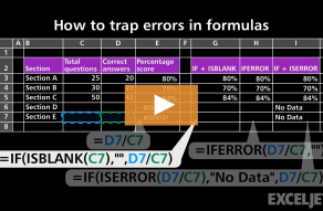
How to trap errors in formulas

What to do when VLOOKUP returns NA
Related functions

ISERROR Function
The Excel ISERROR function returns TRUE for any error type excel generates, including #N/A, #VALUE!, #REF!, #DIV/0!, #NUM!, #NAME?, or #NULL! You can use ISERROR together with the IF function to test for errors and display a custom message, or run a different calculation when an error occurs....

IFNA Function
The Excel IFNA function is a simple way to handle #N/A errors specifically without catching other errors. The IFNA function allows you to specify a custom value or message to display instead of the #N/A error. If no error #N/A error occurs the formula returns a normal result....


