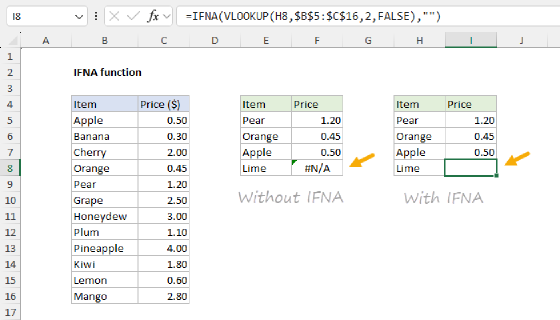
Summary
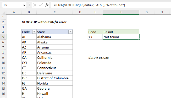
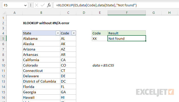
To hide the #N/A error that the XLOOKUP function returns when it can't find a result, you can add a value for the not_found argument. In the example shown, the formula in cell F5 is:
=XLOOKUP(E5,data[Code],data[State],"Not found")
where data is an Excel Table in the range B5:C55. The result is "Not Found" because "XX" does not exist in the Code column.
Generic formula
=XLOOKUP(A1,range1,range2,"Not found")
Explanation
In this example, we have a simple worksheet that uses the XLOOKUP function to lookup the name of a U.S. state when a valid two-letter code is provided as a lookup value. The goal is to remove the #N/A error that XLOOKUP returns when it can't find a result. Although you could use the IFNA or IFERROR function to trap the error and provide an alternative result, the easiest solution is to add a value for the not_found argument, as explained below.
XLOOKUP function
XLOOKUP is a modern replacement for the VLOOKUP function. It is a flexible and versatile function that can be used in a wide variety of situations. In this case, we want to lookup an abbreviation entered in cell E5 and return the correct State name in cell F5, where all data is in an Excel Table named data. We can do this with a formula like this:
XLOOKUP(E5,data[Code],data[State])
Note the lookup_array and return_array are both entered as structured references, which is the name Excel uses for references that refer to parts of an Excel Table. By default, XLOOKUP performs an exact match, so when a valid 2-letter code is entered in cell E5, XLOOKUP will return the corresponding State. For example, if "CO" is entered in cell E5, XLOOKUP will return "Colorado":
XLOOKUP("CO",data[Code],data[State]) // returns "Colorado"
If an invalid code is entered in cell E5, XLOOKUP will return an #N/A error:
XLOOKUP("XX",data[Code],data[State]) // returns #N/A
By the way, this is a good example of how XLOOKUP can easily solve problems that are difficult with VLOOKUP. Because the lookup Code is to the right of State, VLOOKUP can't be used without a more advanced approach. See this example for details.
To extend this formula to provide a custom result when a value is not found, all we need to do is add a value for the not_found argument. In this case, we want to return "Not found", so that is the value we use:
=XLOOKUP(E5,data[Code],data[State],"Not found")
Notice we need to enclose "Not found" in double quotes because it is a text value. To return nothing when XLOOKUP can't find a value, you can provide an empty string ("") like this:
=XLOOKUP(E5,data[Code],data[State],"")
The result from this formula will look like a blank cell when the lookup Code is not found.
XLOOKUP with another formula
The example above displays a custom text message when XLOOKUP returns the #N/A error. However, the alternative value is not limited to text. For example, to have XLOOKUP return zero instead of #N/A, you can use a generic formula like this
=XLOOKUP(A1,range1,range2,0)
In fact, you can provide another formula as well:
=XLOOKUP(A1,range1,range2,formula)
This can be any normal Excel formula, even another XLOOKUP formula that refers to a different set of data. For example, if the first XLOOKUP fails, the second XLOOKUP can try the same lookup in a different table. In this way, you can chain together multiple XLOOKUP formulas.
XLOOKUP with IFNA
XLOOKUP will work fine with other error-trapping formulas like the IFNA function:
=IFNA(XLOOKUP(),alternative)
The IFNA function is a simple way to trap and handle #N/A errors specifically without catching other errors. In the worksheet shown above, you could use IFNA with XLOOKUP like this:
=IFNA(XLOOKUP(E5,data[Code],data[State]),"Not found")
Notice the "Not found" result is now moved out of XLOOKUP into the IFNA function. I can't think of a good reason why you would need to use XLOOKUP with the IFNA function, but it should work just fine. The formula above is not wrong, it is just more complex than necessary.
XLOOKUP with IFERROR
You can also trap #N/A errors returned by XLOOKUP with the IFERROR function like this:
=IFERROR(XLOOKUP(E5,data[Code],data[State]),"Not found")
The IFERROR function is a more general function that will catch any error. This is a different formula from the IFNA formula above, and different from providing a value for the not_found argument. This formula will trap any error returned by XLOOKUP, including #REF!, #NAME, etc. This means there is a risk you might accidentally hide another legitimate error and return a message that is not actually correct. Unless you have a good reason to want this result, I would avoid XLOOKUP with IFERROR.