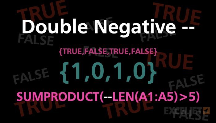
Note: the discussion on this page is about converting TRUE and FALSE values to 1s and 0s. However, the techniques discussed on this page are more general and will also work to convert any number that is text to a numeric value.
In more advanced Excel formulas, you might run into the double negative operation (--):
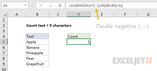
What the heck is that, and what is it doing?
The double negative (sometimes called the even more nerdy "double unary") coerces TRUE or FALSE values to their numeric equivalents, 1 and 0. It's used in formulas where numbers are needed for a particular math operation. That might sound pretty vague, so I'll illustrate with the example above. Let's say you have a list of words in a range, and you want to count how many contain more than 5 characters.
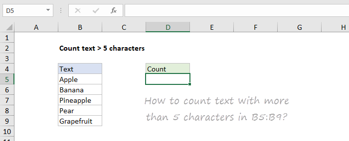
You can build a simple formula to do this with the LEN function and this expression:
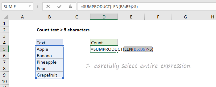
LEN(B5:B9)>5
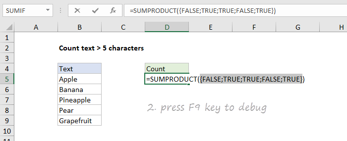
For each of the five cells in the range, LEN will return a character count, which will be checked with >5. The result will be an array of 5 TRUE or FALSE values like this:
{FALSE;TRUE;TRUE;FALSE;TRUE}
Notice there are 3 TRUE values, one each for each text value with more than 5 characters: "banana", "pineapple", and "grapefruit". The 2 FALSE values are for "Apple" and "Pear". Now, if we drop that expression into SUMPRODUCT to count the TRUE results, what do we get?
=SUMPRODUCT(LEN(B5:B9)>5)
We get zero. Why?
Because TRUE and FALSE are logicals, not numbers.
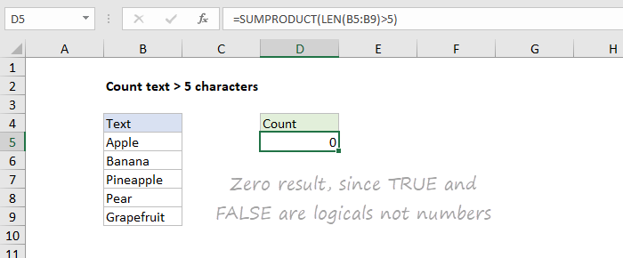
=SUMPRODUCT({FALSE;TRUE;TRUE;FALSE;TRUE}) // returns zero
Excel won't treat logicals as numbers without a little nudge. Fortunately, it doesn't take much. Any math operation will get Excel to convert TRUE to 1 and FALSE to zero. As it turns out, the double negative is a simple and clear way to do this. The first negative will convert TRUE to -1, and the second negative will convert -1 to 1. In the case of FALSE values, the first negative will result in zero, and the second negative will also result in zero.
To use the double negative in this formula, we wrap the original expression in parentheses, put a double negative out front.
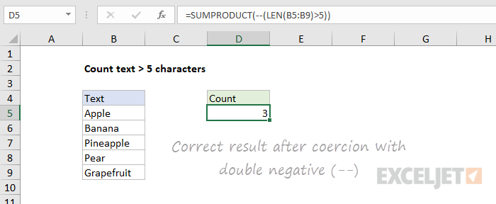
=SUMPRODUCT(--(LEN(B5:B9)>5)) // coerce with --
=SUMPRODUCT({0;1;1;0;1}) // returns 3
By the way, I'm using the SUMPRODUCT function here instead of SUM so that we don't need to enter as an array formula, with control + shift + enter. But SUM entered with control + shift + enter will yield the same result.
Debugging with F9
Whenever you're working with things like double negatives, you must know how to use F9 to debug a formula. The F9 key is like an x-ray to reveal what Excel is really doing "under the hood". For example, if I select the original expression in the formula and press F9, I see an array of TRUE and FALSE values.
If I select the revised formula, including the double negative, and press F9:

Excel will show 1's and 0's.

Video: How to debug a formula with F9
Video: 23 tips to save time with formulas
Other ways to coerce
A double negative is not the only way to get ones and zeros from logicals. You can also add or subtract zero, multiply by one, or use the inscrutably named N function. All of the formulas below will return the same result:
=SUMPRODUCT(--(LEN(range)>5))
=SUMPRODUCT((LEN(range)>5)+0)
=SUMPRODUCT((LEN(range)>5)*1)
=SUMPRODUCT(N(LEN(range)>5))
Which option should you use?
Personally, I use the double negative option most often, because it's simple and clearly indicates the purpose. But I like the N function as well.
Other examples
Coercing TRUE and FALSE values to 1's and 0's is incredibly useful in all kinds of formulas, but it takes a little getting used to. Here are some other formulas that use this technique:
- Count cells that contain errors
- Count cells that contain text case sensitive
- Count cells by day of week
- Cell contains one of many things
- Count matches between columns
- SUMPRODUCT function (see example)
You can find many other examples here.
