Summary
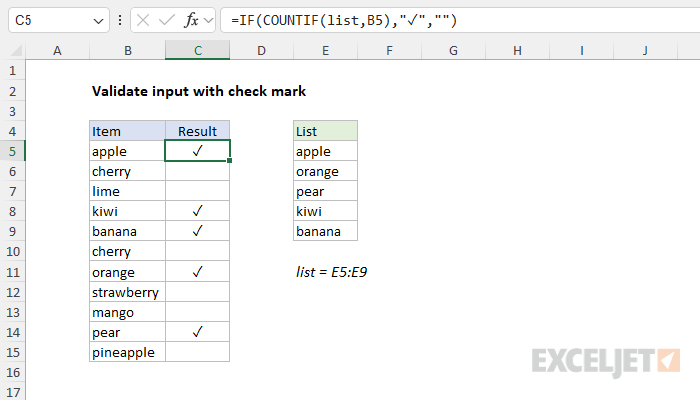
To display a check mark if a value is valid based on an existing list of allowed values, you can use a formula based on the IF function together with the COUNTIF function. In the example shown, the formula in C5 is:
=IF(COUNTIF(list,B5),"✓","")
where list is the named range E5:E9. As the formula is copied down, it returns a checkmark when the value in column B exists in the range E5:E9, and an empty string ("") otherwise.
Generic formula
=IF(logical_test,"✓","")
Explanation
This formula is a good example of nesting one function inside another. At the core, this formula uses the IF function to return a check mark (✓) when a logical test returns TRUE:
=IF(logical_test,"✓","")
If the test returns FALSE, the formula returns an empty string (""). For the logical test, we are using the COUNTIF function like this:
=COUNTIF(list,B5)
COUNTIF returns a count of how many times the value in B5 occurs in the named range list (E5:E9). If the value in B5 exists in the range E5:E9, COUNTIF will return 1. If not, COUNTIF will return zero. Excel's standard behavior is to evaluate any non-zero number as TRUE, and zero as FALSE. So, If the value in B5 exists in E5:E9, COUNTIF returns 1 and IF returns a check mark (✓). If the value in B5 is not found in the allowed list, COUNTIF returns zero and IF returns an empty string (""), which displays nothing.
With hardcoded values
The example above shows allowed values in a range of cells, but allowed values can also be hardcoded into a slightly more complex version of the formula as an array constant like this:
=IF(SUM(COUNTIF(B5,{"red","blue","green"})),"✓","")
Notice that we need to provide the array constant as the criteria, and B5 as the range. This is because COUNTIF will not accept an array constant as the range argument. Because of this change, COUNTIF will return 3 counts (one for each value in the array constant) and we also need to wrap the SUM function around COUNTIF to catch the results from COUNTIF and return a final count.
Note: The fact that COUNTIF won't accept an array for the range argument is not widely understood. To read more about COUNTIF quirkiness, see Excel's RACON functions.
Check mark character (✓)
Inserting a checkmark character in Excel can be surprisingly challenging and you will find many articles on the internet explaining various approaches. The easiest way to get the check mark character (✓) used in this formula into Excel is simply to copy and paste it. If you are copying from this web page, paste it directly into the formula bar to avoid bringing in unwanted formatting. You can also copy and paste directly from the attached worksheet.
If you have trouble with copy and paste, try using the UNICHAR function to insert a checkmark like this:
=UNICHAR(10003) // returns "✓"
UNICHAR (10003) returns a Unicode version of the checkmark: Unicode 2713 (U+2713). The original formula can be written like this:
=IF(COUNTIF(list,B5),UNICHAR(10003),"")
Note: the UNICHAR function was introduced in Excel 2013.
Extending the formula
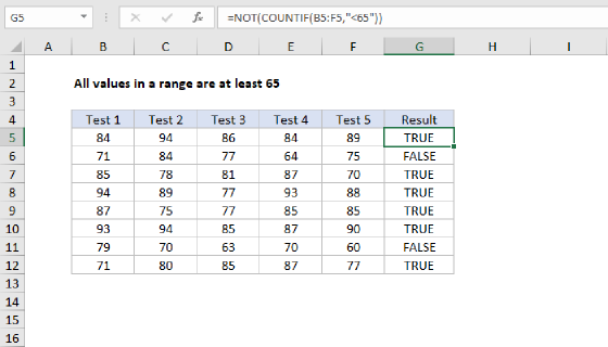
The basic idea in this formula can be extended in many clever ways. For example, the screenshot below shows a formula that returns a check mark only when all test scores are at least 65:
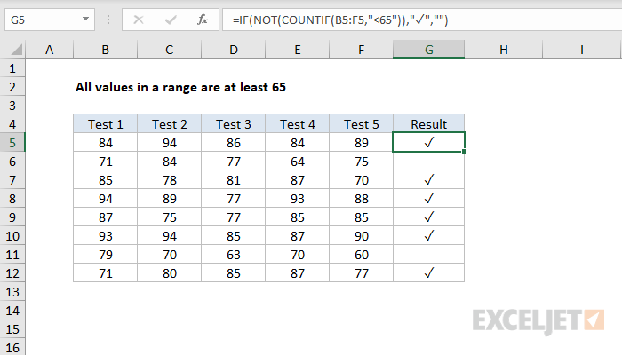
The formula in G5 is:
=IF(NOT(COUNTIF(B5:F5,"<65")),"✓","")
The NOT function reverses the result from COUNTIF. If you find this confusing, you can alternately restructure the IF formula like this:
=IF(COUNTIF(B5:F5,"<65"),"","✓")
In the version of the formula, the logic is more similar to the original formula above. However, we have moved the check mark to the value_if_false argument, so the check mark will appear only if the count from COUNTIF is zero. In other words, the check mark will appear only when no values less than 65 are found.
Note: you can also use conditional formatting to highlight valid or invalid input, and data validation to restrict input to allow only valid data.