Summary
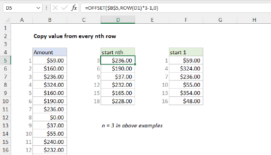
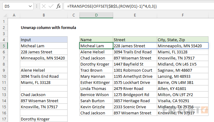
To unwrap a column of values into separate fields, where field values are spaced evenly apart, you can use a formula based on the OFFSET function, with help from the TRANSPOSE function. In the example shown, the formula in D5, copied down, is:
=TRANSPOSE(OFFSET($B$5,(ROW(D1)-1)*4,0,3))
As the formula is copied down, the data is separated into three fields: Name, Street, and City/State/Zip.
Note: In the generic version formula, n represents the number of cells between records, and k represents the number of fields to extract.
This formula requires Excel 2021 or later to work correctly.
Generic formula
=TRANSPOSE(OFFSET($A$1,(ROW(A1)-1)*n,0,k))
Explanation
In this example the goal is to "unwrap" a column of values into separate fields. The values are spaced evenly apart, and the result should be all related values on one row, where each column corresponds to a field of information. The input data appears in column B. Each "record" in the data has three values: Name, Street, and City/State/Zip (combined). New records start every 4th row, and records are separated by an empty cell, which can be thought of as a fourth field that will be ignored. The formula in D5 is:
=TRANSPOSE(OFFSET($B$5,(ROW(D1)-1)*4,0,3))
As this formula is copied down, it extracts the values for each record into cells in a single row.
Note: the formula explained below builds on more basic examples explained here.
Collect fields
Working from the inside out, the core of the solution is the OFFSET function:
OFFSET($B$5,(ROW(D1)-1)*4,0,3)
The OFFSET function is designed to create a reference that is "offset" from a starting point by a given number of rows and columns. In addition, OFFSET has an optional width and height arguments, which specify the size of the reference to be returned.
The starting point inside the OFFSET function is the reference argument, provided as an absolute reference:
=OFFSET($B$5
The reference to B5 is locked so that it won't change as the formula is copied down. The next argument is rows, which indicates the desired row offset from the starting reference. Rather than a hardcoded number, rows is provided as an expression that calculates the required offset:
(ROW(D1)-1)*4 // calculate rows offset
This is where n is provided as 4, in order to reference every fourth value. The ROW function is used to get the row number for cell D1. We start with D1, because we want to start with the number 1. We subtract 1, because we want the first rows offset to be zero. In other words, we want to zero out the rows argument and start with cell B5. As the formula is copied down the column, the value returned by ROW increments by 1, and creates the logic needed to reference every 4th value. See this formula example for a more detailed explanation.
The last two arguments provided to OFFSET are cols and height. Cols is hardcoded as 0 because we want to stay in column B. The height argument is hardcoded as 3, because each record contains 3 cells of information stacked vertically, and we are intentionally ignoring the empty cell between records. As the formula is copied down, the OFFSET function generates the following references:
OFFSET($B$5,(ROW(D1)-1)*4,0,3) // returns B5:B7
OFFSET($B$5,(ROW(D2)-1)*4,0,3) // returns B9:B11
OFFSET($B$5,(ROW(D3)-1)*4,0,3) // returns B13:B15
Transpose fields
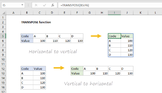
The OFFSET function does almost all of the work in this formula, collecting all three field values for each record. However, the result from OFFSET is a vertical array of values, and we need a horizontal array as a final result. To convert the horizontal array into a vertical array, use the TRANSPOSE function. In the final formula, OFFSET is nested inside TRANSPOSE like this:
=TRANSPOSE(OFFSET($B$5,(ROW(D1)-1)*4,0,3))
OFFSET returns a vertical array like:
{"Micheal Lam";"228 James Street";"Minneapolis, MN 55420"}
And TRANSPOSE catches this array and changes it into a horizontal array like this:
{"Micheal Lam","228 James Street";"Minneapolis, MN 55420"}
Note the commas have replaced the semi-colons. The array is returned to cell D5 and the three values spill into the range D5:F5.