Highlight multiples of specific value

To highlight numbers that are multiples of a another number with conditional formatting, you can use a simple formula based on the MOD function.

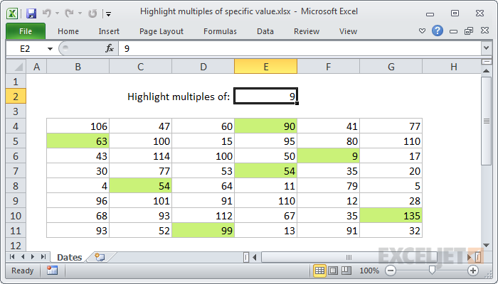
In the example shown, the formula used to highlight multiples of 9 is:

=MOD(B4,$E$2)=0

Note: formula is entered relative to the "active cell" in the selection, cell B4 in this case.

Explanation

Conditional formatting is evaluated for each cell in the range, relative to the upper left cell in the selection. In this case, the formula uses the MOD function to check the remainder of dividing the value in each cell, with the value in cell E2, which is 9. When the remainder is zero, we know that the value is an even multiple of the number 9, so the formula checks the result of MOD against zero.

When MOD returns zero, the expression returns TRUE and the conditional formatting applies. When MOD returns any other result, the expression returns FALSE conditional formatting is not applied.

Note E2 is input as an absolute address ($E$2) to prevent the reference from changing as the conditional formatting rule is evaluated across the selection B4:G11.