Highlight values greater than

Note: Excel contains built-in "presets" for highlighting values above / below / equal to certain values, but if you want more flexibility you can apply conditional formatting with your own formula as explained in this article.

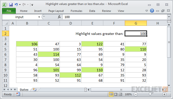
If you want to highlight cells that are "greater than X" with conditional formmatting, you can use a simple formula that returns TRUE when a cell value is greater than X. For example, if you have numbers in the cells B4:G11, and want to highlight cells with a numeric value over 100, you select B4:G11 and create a conditional formatting rule that uses this formula:

=B4>100

It's important that the formula be entered relative to the "active cell" in the selection.

To highlight cells less than 100 with a conditional formatting formula, use:

=B4<100

Explanation

When you use a formula to apply conditional formatting, the formula is evaluated relative to the active cell in the selection at the time the rule is created. So, in this case the formula =B4>100 is evaluated for each of the 40 cells in B4:G11. Because B4 is entered as a relative address, the address will be updated each time the formula is applied. The net effect is that each cell in B4:G11 will be compared to 100 and the formula will return TRUE if the value in the cell is greater than 100. When a conditional formatting rule returns TRUE, the formatting is triggered.

Using a another cell as an input

Note that there is no need to hard-code the number 100 into the rule. To make a more flexible, interactive conditional formatting rule, you can use another cell like a variable in the formula. For example, if you want to use cell G2 as an input cell, you can use this formula:

=B4>$G$2

You can then change the value in cell G2 to anything you like and the conditional formatting rule will respond instantly. Just make sure you use an absolute address to keep the input cell address from changing. Another way to lock the reference is to use a named range, since named ranges are automatically absolute. Just name cell G2 "input" then write the conditional formatting formula like so: