Summary
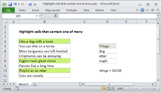
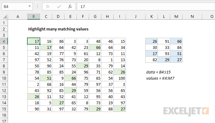
To highlight many matching values in a set of data with conditional formatting you can use a formula based on the COUNTIF function. In the example shown, the formula for green cells is:
=COUNTIF(values,B4)
where values is the named range K4:M7 and the rule is applied to all data in B4:I15.
Generic formula
=COUNTIF(values,A1)
Explanation
In this example, the goal is to highlight all values in K4:M7 (values) that appear in the range B4:I15 (data). The range K4:M7 is named "values" for readability and convenience only. If you don't want to use a named range, use an absolute reference instead.
Although this is a difficult problem for the human eye, it is exactly the kind of thing Excel does very well. The solution above shows matching data in green, and matching values in blue. The colors are applied automatically with conditional formatting and will update instantly if values change. This requires two separate conditional formatting rules, each with its own formula.
Highlight matching data (green)
This formula is based on the COUNTIF function, which takes two arguments: range and criteria and returns a count of values that match criteria. Normally, range represents the cells being checked. For example, to count cells in the range A1:A10 that are equal to 7, you would configure COUNTIF like this:
=COUNTIF(A1:A10,7) // count values = 7
However, in this case, we want to check each cell in B4:I15 against the 12 separate values in K4:M7. One option is to use COUNTIF with values as criteria and use SUM to add up results:
=SUM(COUNTIF(B4,values)) // returns {0,0,0;0,0,1;0,0,0;0,0,0}
Note: the rule is applied to all cells in B4:I15. The relative reference to B4 will change at each cell.
Because we are giving COUNTIF 12 separate numbers to evaluate as criteria, COUNTIF will return 12 counts in an array for each cell in the data. To force a single result, we wrap COUNTIF in the SUM function. Any sum greater than zero means B4 contains a number in values, and any non-zero result will evaluate as TRUE and trigger the rule.
However, a simpler option is to reverse the COUNTIF configuration like this:
=COUNTIF(values,B4) // returns 1
Here, range is values , and B4 is criteria. This gives us a single numeric result – the count of the cell value (B4) in values. As above, any non-zero result means that B4 is a number in K4:M7. And any non-zero result triggers the conditional formatting rule and colors the cell.
Highlight matching values (blue)
The above rule highlights numbers in data that appear in values. We can easily make a rule to highlight cells in values that contain numbers in data. In the example shown, the blue highlighting is created with the following formula:
=COUNTIF(data,K4) // blue highlighting
Notice the approach is the same as above. Each cell in values K4:M7 becomes the criteria argument inside COUNTIF while the range is data (B4:I15). As above, COUNTIF returns a single count for each cell in values and any non-zero result triggers the rule.
Count all matching values
To count the total number of cells in data (B4:I15) that match a number in values (K4:M7) you can use a formula like this:
=SUMPRODUCT(COUNTIF(values,data)) // returns 12
To count the total number of cells in values (K4:M7) that match a value in data (B4:I15), you can use a formula like this:
=SUMPRODUCT(--(COUNTIF(data,values)>0)) // returns 6
Here, because the numbers in values often appear more than once in data, we need to force non-zero counts from COUNTIF to 1 before we add them up, to avoid over counting. We do this by checking if the counts are greater than zero and using a double negative (--) to force the TRUE FALSE results to 1s and 0s.
Note: you can also use the SUM function in place of SUMPRODUCT above, but you will need to enter the formula as an array formula with control + shift + enter, unless you are using Excel 365.