Highlight bottom values

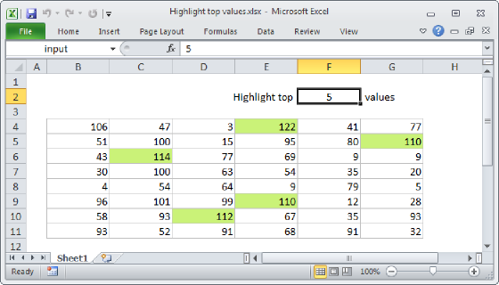
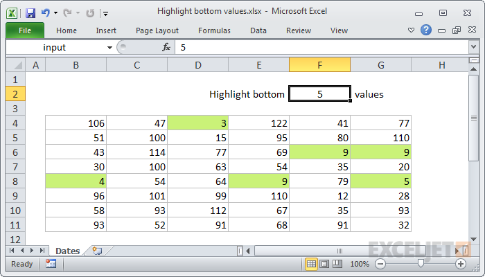
To highlight the smallest (bottom) values in a set of data with conditional formatting, you can use a formula based on the SMALL function. In the example shown, the formula used for conditional formatting is:

=B4<=SMALL(data,input)

where data (B4:G11) and input (F2) are named ranges.

Note: Excel contains a conditional formatting "preset" that highlights bottom values. However, using a formula provides more flexibility.

Explanation

In this example, the goal is to highlight the 5 bottom values in B4:G11 where the number 5 is a variable set in cell F2.

This formula uses two named ranges: data (B4:G11) and input (F2). These are for readability and convenience only. If you don't want to use named ranges, make sure you use absolute references for both of these ranges in the formula.

This formula is based on the SMALL function, which returns the nth smallest value from a range or array of values. The range appears as the first argument in SMALL, and the value for "n" appears as the second:

SMALL(data,input)

In the example, the input value (F2) is 5, so SMALL will return the 5th smallest value in the data, which is 9. The formula then compares each value in the data range with 9, using the less than or equal to operator: