Summary
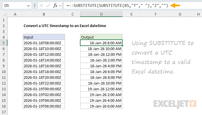
To convert a UTC timestamp to a value that Excel can recognize as a date and time (a datetime), you can use a formula based on the SUBSTITUTE function. In the worksheet shown, the formula in cell D5 looks like this:
=--SUBSTITUTE(SUBSTITUTE(B5,"T"," "),"Z","")
The result in cell D5 is a datetime value that Excel recognizes as January 18, 2026, at 8:00 AM. As the formula is copied down, it converts the other UTC timestamps to datetimes. You can display the datetime as you like with a custom number format. In the example shown, the datetime is displayed with the custom format d-mmm-yy h:mm AM/PM.
UTC timestamps are in Coordinated Universal Time (UTC), which is the same as Greenwich Mean Time (GMT). See below for instructions on how to convert UTC timestamps to a different timezone.
Generic formula
=--SUBSTITUTE(SUBSTITUTE(A1,"T"," "),"Z","")
Explanation
UTC timestamps like 2026-01-18T08:00:00Z are a common standard for representing dates and times, but Excel won't correctly recognize this format without some help. If you try to apply date formatting to a UTC timestamp, nothing happens.
In this example, the goal is to convert UTC timestamps to datetimes that Excel can recognize. In addition, we'll look at how to convert UTC timestamps to datetimes in other time zones.
Table of contents
- What are UTC timestamp?
- About Excel datetimes
- Entering datetimes in Excel
- Converting UTC timestamps with SUBSTITUTE
- Converting UTC timestamps with TEXTSPLIT
- Converting UTC timestamps to other time zones
- Summary
What are UTC timestamps?
UTC timestamps are a standard format for representing dates and times. This format is a text value that conforms to the ISO 8601 standard for representing dates and times. The generic format is YYYY-MM-DDTHH:MM:SSZ which looks like this: 2026-01-18T08:00:00Z. The "T" separates the date from the time, and the "Z" at the end stands for "Zulu time", which is another name for UTC (Coordinated Universal Time), also known as Greenwich Mean Time (GMT).
You'll run into UTC timestamps when you're working with data from APIs, web services, databases, and data exports. They're popular because they're unambiguous – there's no confusion about whether 01/02/2026 means January 2nd or February 1st, and the timezone (GMT) is also known.
The problem with UTC timestamps is that Excel doesn't recognize them as dates. If you paste a UTC timestamp into a cell and try to format it as a date, nothing happens. The same is true if you try a function like MONTH or YEAR. Excel just sees text, not a date.
About Excel datetimes
In Excel, dates are large serial numbers starting on January 1, 1900. The date January 1, 1900 is the serial number 1, January 2, 1900 is the serial number 2, and so on. The date January 1, 2026 is represented as the serial number 46023. Because each date is a number, and there are 24 hours in a day, Excel times are fractions of a day. The time 12:00 AM is represented as the decimal value 0. The time 12:00 PM is the decimal value 0.5. The time 6:00 PM is the decimal value 0.75.
Although many users don't realize it, dates with times are stored as a single number in a cell. For example, January 18, 2026 12:00 PM is stored in Excel as the number 46040.5. This is referred to as a "datetime" value - a single number that represents both a date and a time. Because the UTC timestamp contains both a date and a time, our goal is to convert the UTC timestamp to a datetime value that Excel can recognize.
Tip: A good way to check datetimes in Excel is to temporarily format them using the General number format (the shortcut is Ctrl + Shift + ~). This will let you see the number that represents the date and time.
Entering datetimes in Excel
One way to enter a datetime in Excel is to use a formula based on the DATE and TIME functions. For example, to enter the datetime January 18, 2026 at 12:00 PM, you can use a formula like this:
=DATE(2026,1,18)+TIME(12,0,0)
This formula returns the datetime value January 18, 2026 at 12:00 PM (46040.5). Of course, most users will enter the date and times manually by typing the date and time in a cell. The trick is to enter the date and time separated by a space. For example, to enter January 18, 2026 at 12:00 PM, type 18-Jan-2026 12:00 PM, and Excel will automatically convert the text to a datetime value. Importantly, you can also enter a datetime in the UTC format by removing the "T" and "Z".
2026-01-18 12:00:00 // YYYY-MM-DD HH:MM:SS
Excel will correctly understand this as a datetime value. To summarize, if we remove the "T" and "Z" from the UTC timestamp, Excel will be able to interpret it as a valid datetime. This is the approach we will take in the following examples.
Tip: you can also enter a format like
1/18/2026 12:00 PMor18/1/2026 12:00 PMdepending on your regional settings. However, this can be confusing and ambiguous and result in incorrect dates. A format like2026-01-18 12:00 PMor2026-01-18 12:00avoids this confusion.
Converting UTC timestamps with SUBSTITUTE
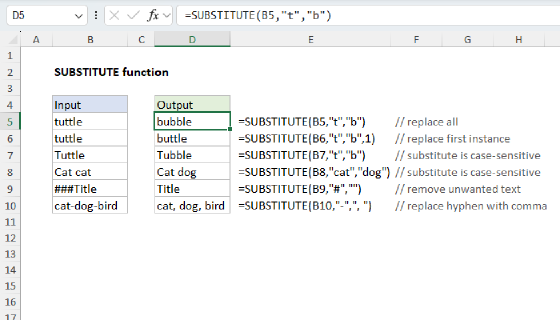
Since we want to remove the 'T' and the 'Z' from the UTC timestamp, one solution is to use the SUBSTITUTE function. The SUBSTITUTE function replaces text in a text string with another text string. To replace the "T" with a space, and to remove the "Z" altogether, we can use SUBSTITUTE like this:
=SUBSTITUTE(B5,"T"," ") // replace the "T" with a space
=SUBSTITUTE(B5,"Z","") // remove the "Z"
Note in the second formula, we are removing the "Z" altogether by using an empty string (""). By nesting the two SUBSTITUTE functions together, we can remove both the "T" and the "Z" in a single formula:
=SUBSTITUTE(SUBSTITUTE(B5,"T"," "),"Z","") // remove both the "T" and the "Z"
The inner SUBSTITUTE function replaces the "T" with a space and hands the result to the outer SUBSTITUTE function, which then replaces the "Z" with an empty string. The final result is the text string "2026-01-18 08:00:00" without the "T" and "Z".
You might think we are done at this point, but we aren't quite finished. If you use the formula above, Excel will simply return the text string without recognizing it as a date/time value. The final step is to give Excel a little kick in the butt to make it evaluate the text string as a number. One trick is to use the double negative operator (--). This is the final formula in cell D5:
=--SUBSTITUTE(SUBSTITUTE(B5,"T"," "),"Z","")

The double negative (--, also called double unary) is a simple math operation that causes Excel to try to interpret the text string as a number. The result is the datetime value January 18, 2026 at 8:00 AM (46040.3333333333). To display that date and time together, we are using the custom number format d-mmm-yy h:mm AM/PM.
Excel's laziness here isn't really surprising. SUBSTITUTE is a text function, and it returns a text string, so Excel leaves it alone. The only thing worse than a lazy Excel is a hyper Excel that converts values without asking.
Converting UTC timestamps with TEXTSPLIT
Of course, since this is Excel, there is always another way to solve the problem. Another way to convert the UTC timestamp to a datetime value is to use the TEXTSPLIT function. TEXTSPLIT splits a text string into an array of values based on a delimiter. One interesting feature of TEXTSPLIT is that the delimiter itself is lost in the process. For example, if we use TEXTSPLIT to split the UTC timestamp with the "T" as the delimiter, we get an array with two separate values, the date and the time.
=TEXTSPLIT(B5,"T") // returns {"2026-01-18","08:00:00Z"}
Note that the "T" is lost in the process. We can actually go one step further and split the UTC timestamp with the "T" and "Z" as the delimiters in a single formula:
=TEXTSPLIT(B5,{"T","Z"},,1) // returns {"2026-01-18","08:00:00"}
Note that we have provided the delimiters as an array constant and also set ignore_empty to 1 (TRUE). We need to set ignore_empty to TRUE to prevent TEXTSPLIT from returning an array with three values: {"2026-01-18","08:00:00",""}, which comes from the "Z" delimiter.
Okay, so at this point, the formula above will split the UTC timestamp into two values: the date and the time. How can we bring them back together again? Since our goal is to get a single numeric value in the end, it's actually pretty simple. We can simply wrap the formula in the SUM function like this:
=SUM(--TEXTSPLIT(B5,{"T","Z"},,1))
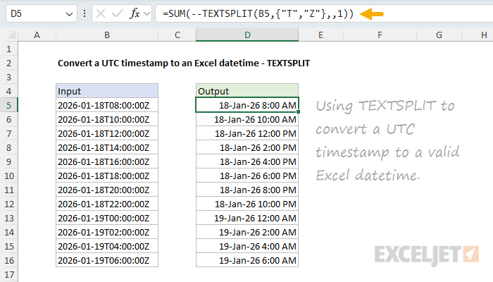
Notice we are using the double unary operator (--) trick again to convert the text strings returned by TEXTSPLIT to numbers before adding them together. The result is the datetime value January 18, 2026 at 8:00 AM (46040.3333333333).
Is this formula better than the SUBSTITUTE formula? Well, it's certainly more clever, but it's also more complex. But I think it is also a good learning formula because it brings together many important concepts at once. It also manages the date and time separately, which might be convenient in some situations.
Converting UTC timestamps to other time zones
In the previous examples, we converted the UTC timestamp to a datetime value in the UTC timezone, also known as Greenwich Mean Time (GMT). But what if you need to convert the UTC timestamp to a datetime value in a different timezone, like the Pacific Standard Time (PST) timezone?
To do this, we need to know the offset between the UTC timezone and the target timezone. For example, the offset between the UTC timezone and the Pacific Standard Time (PST) timezone is -8 hours. This means that when the UTC timestamp is 8:00 AM, the Pacific Standard Time (PST) timestamp is 12:00 AM. The offset is negative because the Pacific Standard Time (PST) timezone is 8 hours behind the UTC timezone.
To convert the UTC timestamp to a datetime value in the Pacific Standard Time (PST) timezone, we can use either formula below:
=--SUBSTITUTE(SUBSTITUTE(B5,"T"," "),"Z","") - TIME(8,0,0)
=SUM(--TEXTSPLIT(B5,{"T","Z"},,1)) - TIME(8,0,0)
Note that both formulas are based on the examples above. You can see how this works in the screenshot below, where we have converted the UTC timestamp to a datetime value in the Pacific Standard Time (PST) timezone with the TEXTSPLIT option:
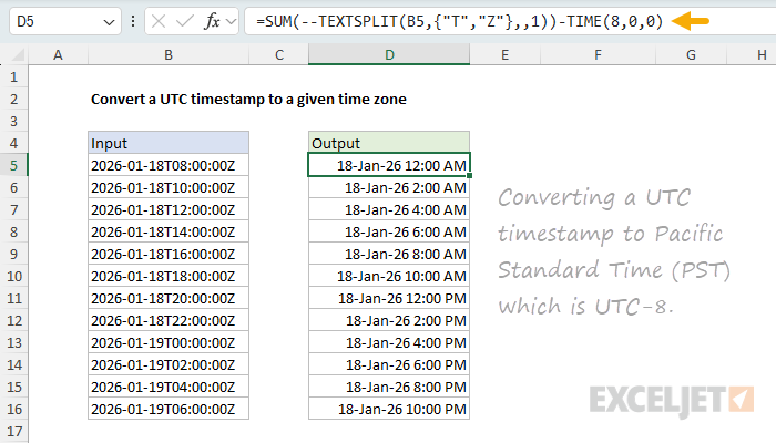
The time zone conversion is handled with the TIME function, which creates a time value of 8 hours. We simply subtract this time value from the result to get the datetime value in the Pacific Standard Time (PST) timezone. To convert to Eastern Standard Time (EST), which is UTC-5, we can simply subtract 5 hours from the result:
=--SUBSTITUTE(SUBSTITUTE(B5,"T"," "),"Z","") - TIME(5,0,0)
=SUM(--TEXTSPLIT(B5,{"T","Z"},,1)) - TIME(5,0,0)
Summary
UTC timestamps are a common format for dates and times in data exports, APIs, and other systems. They look like this: "2026-01-18T08:00:00Z". The problem is that Excel doesn't recognize this format as a date. If you try to apply date formatting to a UTC timestamp, nothing happens. Fortunately, if you strip out the "T" and "Z", Excel will recognize what's left as a valid datetime. The SUBSTITUTE approach is simple and works in all versions of Excel:
=--SUBSTITUTE(SUBSTITUTE(B5,"T"," "),"Z","")
The TEXTSPLIT approach is a bit more clever, and a good way to learn about delimiters and array handling:
=SUM(--TEXTSPLIT(B5,{"T","Z"},,1))
Both formulas use the double negative (--) trick to force Excel to evaluate the text as a number. Once you have a proper datetime value, you can format it as you like and adjust for timezone offsets by adding or subtracting hours with the TIME function.