Summary
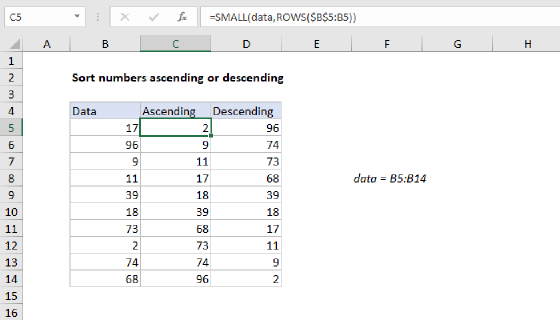
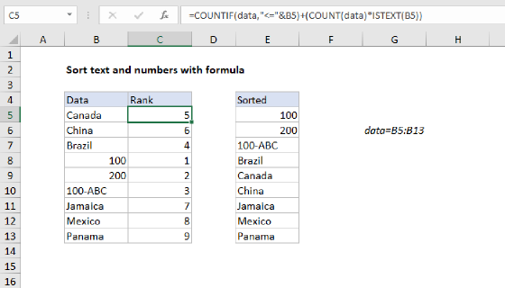
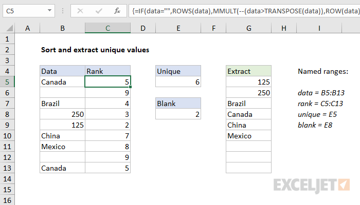
To dynamically sort and extract unique values from a list of data, you can use an array formula to establish a rank in a helper column, then use a specially constructed INDEX and MATCH formula to extract unique values. In the example shown, the formula to establish rank in C5:C13 is:
=IF(data="",ROWS(data),MMULT(--(data>TRANSPOSE(data)),ROW(data)^0))
where "data" is the named range B5:B13.
Note: this is a multi-cell array formula, entered with control + shift + enter.
Generic formula
=MMULT(--(data>TRANSPOSE(data)),ROW(data)^0)
Explanation
Note: the core idea of this formula is adapted from an example in Mike Girvin's excellent book Control+Shift+Enter.
The example shown uses several formulas, which are described below. At a high level, the MMULT function is used to compute a numeric rank in a helper column (column C), and this rank is then used by an INDEX and MATCH formula in column G to extract unique values.
Ranking data values
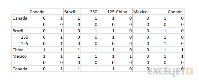
The MMULT function performs matrix multiplication and is used to assign a numeric rank to each value. The first array is created with the following expression:
--(data>TRANSPOSE(data))
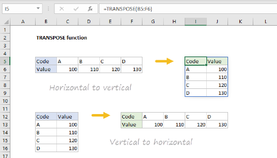
Here, we use the TRANSPOSE function to create a horizontal array of data, and all values are compared to one another. In essence, each value is compared against every other value to answer the question "is this value greater than every other value". This results in a two-dimensional array, 9 columns x 9 rows, filled with TRUE and FALSE values. The double negative (--) is used to coerce the TRUE FALSE values to 1s and zeros. You can visualize the resulting array like this:
The matrix of 1s and zeros above becomes array1 inside the MMULT function. Array2 is created with this expression:
ROW(data)^0
Here, each row number in "data" is raised to the power of zero to create a one-dimensional array, 1 column x 9 rows, filled with the number 1. MMULT then returns the matrix product of the two arrays, which become the values seen in the rank column.
We get back all 9 rankings at the same time in an array, so we need to put the results into different cells all at once. Otherwise, each cell will only show the first ranking value in the array that is returned.
Note: this is a multi-cell array formula, entered with control + shift + enter, in the range C5:C13.
Handling blank cells
Empty cells are handled with this part of the ranking formula:
=IF(data="",ROWS(data)
Here, before we run MMULT, we check if the current cell in "data" is blank. If so, we assign a rank value that equals the row count in data. This is done to force blank cells to the bottom of the list, where they can easily be excluded later as unique values are extracted (explained below).
Counting unique values
To count unique values in the data, the formula in E5 is:
=SUM(--(FREQUENCY(rank,rank)>0))-(blank>0)
Since the ranking formula above assigns a numeric rank to each value, we can use the FREQUENCY function with SUM to count unique values. This formula is explained in detail here. We then subtract 1 from the result if there are any empty cells in the data:
-(blank>0)
where "blank" is the named range E8, and contains this formula:
=COUNTBLANK(data)
Essentially, we reduce the unique count by one if there are blank cells in the data, since we don't include these in results. The unique count in cell E5 is named "unique" (for unique count), and is used by the INDEX and MATCH formula to filter out blank cells (described below).
Extracting unique values
To extract unique values, G5 contains the following formula, copied down:
=IF(ROWS($G$5:G5)>unique,"",INDEX(data,MATCH(MIN(IF(ISNA(MATCH(data,$G$4:G4,0)),rank)),rank,0)))
Before we run the INDEX and MATCH formula, we first check if the current row count in the extraction area is greater than the unique count the named range "unique" (E5):
=IF(ROWS($G$5:G5)>unique,"",
If, so, we are done extracting unique values and we return an empty string (""). If not, we run the extraction formula:
INDEX(data,MATCH(MIN(IF(ISNA(MATCH(data,$G$4:G4,0)),rank)),rank,0))
Note there are two MATCH functions here, one inside the other. The inner MATCH uses an expanding range for an array and the named range "data" for the lookup value:
MATCH(data,$G$4:G4,0)
Notice the expanding range begins on the "row above", row 4 in the example. The result from the inner MATCH is an array which, for each value in data, contains either a numeric position (the value has already been extracted) or the #N/A error (the value has not yet been extracted). We then use IF and ISNA to filter these results, and return the rank value for all values in "data" not yet extracted:
IF(ISNA(results),rank))
This operation results in an array, which is fed into the MIN function in order to get the "minimum rank value" for data values not yet extracted. The MIN function returns this value to the outer MATCH as a lookup value and the named range "rank" as the array:
MATCH(min_not_extracted,rank)),rank,0)
Finally, MATCH returns the position of the lowest rank value to INDEX as a row number, and INDEX returns the data value in the current row of the extraction range.
UNIQUE and SORT in Excel 365
In Excel 365, the UNIQUE and SORT functions provide a more elegant way to list unique values and count unique values. These formulas can be adapted to apply logical criteria, and SORT can be combined with UNIQUE.