Summary
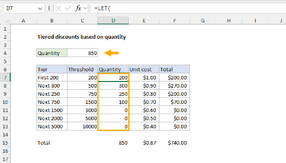
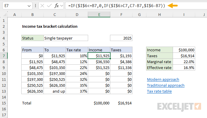
To calculate the total income tax owed in a progressive tax system with multiple tax brackets, you can use a simple, elegant approach that leverages Excel's new dynamic array engine. In the worksheet shown, the main challenge is to split the income in cell I6 into the correct tax brackets. This is done with a single formula like this in cell E7:
=LET(
income,I6,
upper,C7:C13,
lower,DROP(VSTACK(0,upper),-1),
IF(income<=lower,0,
IF(income>upper,upper-lower,income-lower))
)
This formula splits the income into the seven brackets in column E in one step. After that, simple formulas can be used to compute the tax per bracket and total tax. As explained below, it is also possible to extend this formula to calculate all taxes in one step.
Note: Because this formula uses new functions like LET, DROP, and VSTACK, it requires a current version of Excel. In older versions of Excel, you can use a more traditional formula approach. Both methods are explained below.
Explanation
In this example, the goal is to calculate the total income tax owed in a progressive tax system with multiple tax brackets, as shown in the worksheet. The article below first reviews how taxes are computed in a progressive system. Next, it shows how to accomplish this task in Excel using two different methods:
- A modern approach that leverages the latest Excel formulas and functions
- A traditional approach that works in older versions of Excel.
The main focus of this article is a method to split income out by tax bracket in column E so that taxes can easily be computed in column F. However, it also discusses a single formula solution to calculate all taxes in one step in cell I7. The article also explains how to make the tax rates dynamic based on the taxpayer's status in cell C4 and the year selected in F4.
New: I've updated the worksheet to include tax rates for the year 2025. I've also modified the worksheet to store tax rates for previous years and fetch the correct rates for a given year based on the user's year selection in F4.
Table of Contents
- Instructions
- About progressive tax brackets
- Tax calculation with multiple brackets
- Method 1 - A modern and elegant approach
- Single formula option
- Marginal vs. Effective Tax Rates
- Method 2 - A traditional formula approach
- Clever MIN and MAX alternative
- Dynamic tax brackets
- How to update the worksheet with new tax rates
Instructions
Download the attached Excel workbook. The formulas in Sheet1 require a current version of Excel (Excel 365 or Excel 2024). The formulas in Sheet2 should work in any version. The worksheets require only three inputs:
- Select your filing status using the dropdown in C4.
- Select the tax year using the dropdown in cell F4.
- Enter your taxable income in cell I6.
Sheet3 contains U.S. federal tax rates for the years 2023, 2024, and 2025. Sheet1 and Sheet2 calculate the taxes in different ways, but given the same inputs, the results should be the same.
About progressive tax brackets
The U.S. has a progressive tax system, which means that as your income increases, so does the rate at which you're taxed. Instead of taxing all income at a single rate, income is split into different "brackets," with each portion taxed at a different rate. The more you earn, the more income falls into higher brackets, which have a progressively higher rate. The IRS publishes brackets and tax rates each year. For 2025, the tax rates for a single taxpayer look like this:
| Tax rate | on taxable income from... | up to... |
|---|---|---|
| 10% | $0 | $11,925 |
| 12% | $11,926 | $48,475 |
| 22% | $48,476 | $103,350 |
| 24% | $103,351 | $197,300 |
| 32% | $197,301 | $250,525 |
| 35% | $250,526 | $626,350 |
| 37% | $626,351 | And up |
Note: I don't know why the IRS adds $1.00 to the "From" values. This may *look* correct, but it isn't mathematically correct and may cause you to "lose" 1 dollar of income in some brackets. To keep things simple and avoid confusion, I have removed the extra $1.00 in the worksheet example. For the same reason, the "modern" formulas below ignore the "From" values and generate their own lower thresholds directly using the "To" values.
Tax calculation with multiple brackets
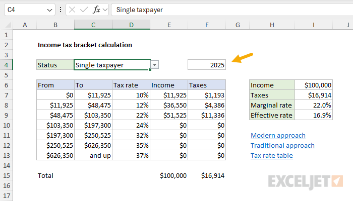
Taxes are calculated progressively through the brackets. For example, for a single filer with $100,000 of taxable income in 2025, the total tax owed is calculated as follows:
- In the first bracket, from $0 to $11,925, $11,925 is taxed at 10% = $1,193.
- In the second bracket, from $11,925 to $48,475, $36,550 is taxed at 12% = $4,386.
- In the third bracket, from $48,475 to $103,350, $51,525 is taxed at 22% = $11,336.
- Since $100,000 does not exceed $103,350, no portion is taxed at 24%.
The total tax is $16,915, with each portion of income taxed at progressively higher rates. The marginal tax rate is 22%, and the effective tax rate is 16.9%.
Method 1 - A modern and elegant approach
First, let's solve this problem in a fun, modern way. The hard part of this problem is splitting the income by bracket. These are the numbers seen in the range E7:E13. To be clear, the math is simple, but implementing the math using cell references can be tricky. In the worksheet shown, the formula used in cell E7 is:
=LET(
income,I6,
upper,C7:C13,
lower,DROP(VSTACK(0,upper),-1),
IF(income<=lower,0,
IF(income>upper,upper-lower,income-lower))
)
This formula returns the correct income per bracket for all seven brackets at once. Compared to traditional formulas, it has several notable advantages:
- Just one formula, so there is no need to copy and paste.
- Only two cell references are required.
- There is no need to lock references due to the magic of dynamic arrays.
- Only the upper limits are required. The lower limits are generated automatically.
- Variable names that make the formula easier to read and understand.
Let's walk through how the formula works step by step. First, to make the formula more readable and efficient by storing and reusing values, the LET function defines three variables:
=LET(
income,I6,
upper,C7:C13,
lower,DROP(VSTACK(0,upper),-1),
- income: This is the income to be taxed, coming from cell I6.
- upper: The "upper" limits of the tax brackets, from range C7:C13.
- lower: This creates the "lower" limits of the tax brackets. (see below)
The lower limits are generated with the VSTACK function and the DROP function like this:
DROP(VSTACK(0,upper),-1)
The values in upper are from the range C7:C13. In array form, they look like this:
{11925;48475;103350;197300;250525;626350;"And up"}
Inside DROP, VSTACK is used to add a zero (0) as the first value:
=VSTACK(0,upper)
The result is an array like this:
{0;11925;48475;103350;197300;250525;626350;"And up"}
This array is returned directly to the DROP function, which is configured to remove the last row:
=DROP({0;11925;48475;103350;197300;250525;626350;"And up"},-1)
The result is a new array without the "And up" value:
{0;11925;48475;103350;197300;250525;626350}
At this point, we have the upper and lower arrays correctly aligned and are ready to implement the logic.
Note: I could have picked up the lower values directly from the range B7:B13. However, I wanted this formula to work when only the upper threshold brackets are available. Because the formula uses the upper values to derive the lower values, the values in B7:B13 can be removed, and the formula will continue to operate correctly.
Next, we get to the heart of the formula, which is based on a nested IF function.
IF(income<=lower,0,
IF(income>upper,upper-lower,income-lower))
The key to understanding this code is to remember that we are processing an array of values, not just a single value. Because the upper and lower arrays each contain seven values, the formula will return seven results that will "flow" through the nested IF according to the following logic:
- If the income is less than or equal to the lower bound of a bracket, then no income falls within that bracket, so the tax contribution from this bracket is 0.
- If the income is greater than the upper limit of the current bracket, the result is the difference between the upper and lower limits (upper - lower), which represents the full taxable portion for that bracket.
- Otherwise, the result is the difference between the income and the lower limit (income - lower), which is the portion of the income that falls within that bracket.
In summary, the formula uses the upper limits in C7:C13 to compute the correct lower limits. Then, it uses the IF function and the upper and lower limits to split the income in cell I6 into the correct brackets. Once the income is split by bracket, we can easily calculate the tax per bracket with a formula like this in cell F7:
=D7:D13*E7:E13
This formula simply multiplies the tax rates in D7:D13 by the income splits in E7:E13. The result is an array of 7 values like this, which spill into F7:F13:
{1193;4386;11336;0;0;0;0}
To compute the total taxes owed in F15, we use the SUM function:
=SUM(F7:F13)
The formula in E15 serves as a sanity check to make sure that all income from I6 has been accounted for:
=SUM(E7:E13)
Single formula option
So far, we have calculated the tax per bracket and total tax with separate formulas that return "per bracket" results on the worksheet. This is a good approach because it makes it easy to validate results at any point. But what if you want to calculate the total taxes owed in a single formula? In that case, we need to add a few more lines of code to our formula. Below is the formula in cell I7, which does everything in one step:
=LET(
income,I6,
tax_rates, D7:D13,
upper,C7:C13,
lower,DROP(VSTACK(0,upper),-1),
income_by_bracket,IF(income<=lower,0,
IF(income>upper,upper-lower,income-lower)),
tax_by_bracket,income_by_bracket*tax_rates,
SUM(tax_by_bracket)
)
This new formula extends the original formula by adding three new variables:
- tax_rates - the range D7:D13
- income_by_bracket - defined by the nested IF code explained above
- tax_by_bracket - defined by income_by_bracket * tax_rates
Then, on the last line, we use the SUM function to return a result by summing the amounts in tax_by_bracket:
SUM(tax_by_bracket)
This result matches the value in cell F15. Next, let's look at how to calculate the marginal and effective tax rates.
Marginal vs. Effective Tax Rates
When discussing income tax, there are two rates you are likely to encounter: the marginal tax rate and the effective tax rate. The marginal tax is the tax rate applied to the last dollar earned. For $100,000 of income, the marginal tax rate is 22% since that's the rate applied to income in the third bracket. The effective tax is the overall percentage of income paid in taxes. It's calculated by dividing the total tax ($16,915) by the total income ($100,000), which gives an effective tax rate of 16.9%. This demonstrates that while the highest rate paid on the last portion of income is 22%, the average rate across all brackets is lower due to the progressive system. To compute the marginal tax rate in cell I8, we use the XLOOKUP function like this:
=XLOOKUP(I6,C7:C13,D7:D13,,1)
- lookup_value - from I6
- lookup_array - the upper values in C7:C13
- return_array - the tax rates in D7:D13
- if_not_found - omitted
- match_mode - 1, for an exact match or next largest
The key here is the setting for match_mode (1), which causes XLOOKUP to return the next largest tax rate when an exact match on income is not found. To compute the effective tax rate in I9, we divide the total computed tax in I7 by the taxable income in I6:
=I7/I6
The results from both formulas are formatted using Excel's percentage number format.
Method 2 - A traditional formula approach
In older versions of Excel that do not support dynamic array formulas, I think the easiest solution is to use the "From" values directly in your calculations, then use the same nested IF logic explained above to compute the income by bracket. You can see this approach in the worksheet below:
As mentioned above, the main challenge is to split the income in cell I6 by bracket in a clean and simple way. This is done with the following formula in cell E7:
=IF($I$6<=B7,0,IF($I$6>C7,C7-B7,$I$6-B7))
As the formula is copied down, the income in each bracket is calculated like this:
- If the income in I6 is less than or equal to the lower bound in B7, then no income falls within that bracket, so the tax contribution from this bracket is 0.
- If the income in I6 is greater than the upper limit (C7), the result is the difference between the upper and lower limits (C7 - B7). This is the full taxable portion for that bracket.
- Otherwise, the result is the difference between the income and the lower limit (I6 - B7), which is the remaining portion of the income that falls within that bracket.
Then, to calculate the tax in each bracket, multiply the tax rate by the income in cell F7:
=D7*E7
As this formula is copied down column F, it returns the correct income tax in each bracket.
Clever MIN and MAX alternative
If you like clever formulas, you can simplify the nested IF logic above by replacing it with a more compact alternative based on MAX and MIN like this:
=MAX(0,MIN($I$6,C7)-B7)
Both formulas apply the same logic and return the same results.
Dynamic tax brackets
Retrieving the correct tax rates for a given filing status and year isn't the main focus of splitting income into tax brackets and calculating the tax in each bracket. However, it's an important part of this worksheet's design, so I want to explain how it's done. The lookup formulas below are advanced. They are built on the idea that you can use numeric indexes for lookup operations that need to change based on specific inputs. For example, "Married filing jointly" is item 2 in the list of status options. The main idea is that we can do something intelligent with the number 2, when the user has made that selection. Specifically, we want to retrieve columns 4 and 5 when the filing status is 2. The trick is working out the simple math operations needed to convert the 2 into a 4 and 5. If you haven't been exposed to this idea before, don't be discouraged. Learning how to design and implement formulas like this takes time and practice. See this page for a simplified example with a more detailed explanation.
The formulas explained above split income into brackets and apply the correct tax rates. However, we still need to adapt the worksheet to make the tax rates reflect user choices. This is an advanced lookup scenario, and it requires careful design. The goal is to dynamically retrieve the correct tax rate data based on the selected year and filing status. The screen below shows how this information is organized on Sheet3 of the workbook, and the orange numbers represent the numeric index values we can use:
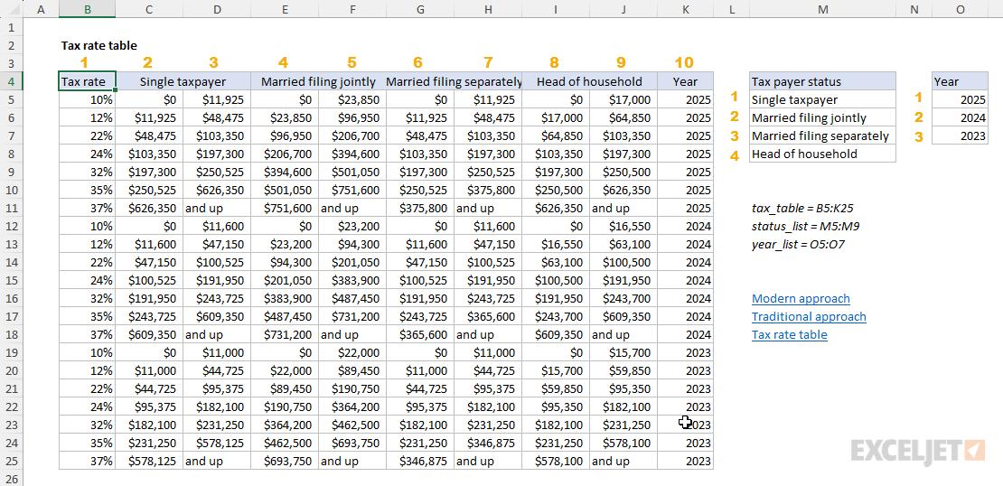
The tax rates for all years are stored in the range B5:K25. This table contains ten columns in total. The first column contains the tax rate brackets. The next eight columns contain the thresholds for each filing status. Notice each filing status has a pair of columns, one for "From" values and one for "To" values. The last column is Year, which contains the year the brackets were active. There are seven brackets, so seven rows for each year. For convenience, tax_table (B5:K25), status_list (M5:M9), and year_list (O5:O7) are named ranges used by the formulas that fetch rates.
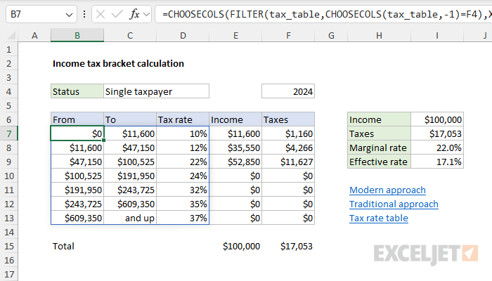
Back on Sheet1, cell C4 contains a dropdown list that presents values from the status_list. Cell F4 is a similar dropdown list that lets the user select the year from year_list. Both dropdowns are created with Data Validation. The values selected in C4 and F4 drive the formulas that retrieve the correct tax rates for the selected year and filing status. On Sheet1, the formula in B7 retrieves all required data in one step like this:
=CHOOSECOLS(
FILTER(tax_table,CHOOSECOLS(tax_table,-1)=F4),
XMATCH(C4,status_list)*2,
XMATCH(C4,status_list)*2+1,1)
At a high level, we are using the CHOOSECOLS function to get the columns we need based on the filing status. However, before we get the columns, we use the FILTER function to get tax rates for the selected year like this:
FILTER(tax_table,CHOOSECOLS(tax_table,-1)=F4) // get rates for year
FILTER is configured to return tax rate data for a given year like this:
- array - the named range tax_table (B5:K18 on sheet3)
- include - CHOOSECOLS(tax_table,-1)=F4
The tricky part is using CHOOSECOLS with a -1 to get the last column of the tax table, which is compared to cell F4. The result from FILTER is the subset of the tax rates that correspond to the year in F4. This is delivered directly to the outer CHOOSECOLS function as the array argument. We now have all tax rate data for a given year, but we still have three tricky steps remaining:
- Calculate a numeric index for the "From" and "To" columns for the selected filing status.
- Extract the two columns related to filing status plus the tax rates themselves.
- Reorder the extracted columns to match the order on Sheet1 (rates appear last).
For step 1, we can use the selected status value as a numeric index, but we must make adjustments to account for the fact that each status has two columns. To get an index for the "From" column, we use the XMATCH function like this:
XMATCH(C4,status_list)*2
We multiply the result by 2, since each tax status has two columns, starting with column 2. To get an index for the "To" column, we use XMATCH again in the same way:
XMATCH(C4,status_list)*2+1
This time, we multiply the result from XMATCH by 2, and then we add 1 to account for the fact that the To" column is the "next" column in each category. To recap, the XMATCH formulas above give us the numeric index number for each of the two columns we need for filing status. When the status is "Single taxpayer", the first XMATCH returns 2 and the second returns 3. Then, to get the last column (tax rates), we simply hardcode the number 1 since this data is the first column of the tax table. Putting the 1 last also effectively reorders the columns as needed, knocking off Step 3 from above. The result inside CHOOSECOLS looks like this:
=CHOOSECOLS(array,2,3,1)
When a user selects a different taxpayer status, XMATCH calculates new column indexes. For example, if we choose "Married filing jointly", the "From" column becomes 4, the "To" column becomes 5, and the tax rate remains unchanged as 1.
=CHOOSECOLS(array,4,5,1)
Traditional formula option
In older versions of Excel, we don't have functions like FILTER or CHOOSECOLS to use. One alternative is to use the OFFSET function with the MATCH function. In Sheet2, the formula in B7 retrieves the correct "From" and "To" columns in one step like this:
=OFFSET(tax_table,7*(MATCH(F4,year_list,0)-1),MATCH(C4,status_list,0)*2-1,7,2)
Note: This is a multi-cell array formula entered in the range B5:C13 with control + shift + enter.
This formula extracts a 7-row by 2-column range from the tax_table based on the taxpayer status and year selected. The tricky part is calculating the right offsets for the selected year and status. The inputs to OFFSET look like this:
- reference - tax_table (OFFSET will use the upper left cell)
- rows - 7*(MATCH(F4,year_list,0)-1)
- cols - MATCH(C4,status_list,0)*2-1
- height - 7 (hardcoded)
- width - 2 (hardcoded)
To calculate the rows offset, we use MATCH like this:
7*(MATCH(F4,year_list,0)-1
If F4 = 2025, MATCH returns 1 (since 2025 is in the first row). If F4 = 2024, MATCH returns 2 (since 2024 is in the second row). Therefore:
- For 2025 (MATCH result = 1) → 7 * (1-1) = 0 → Stays in rows 5-11.
- For 2024 (MATCH result = 2) → 7 * (2-1) = 7 → Moves down 7 rows to rows 12-18.
To calculate the column offset, we use MATCH like this:
MATCH(C4,status_list,0)*2-1
Here, we multiply the MATCH result by 2, then subtract 1 because we need to skip the first column and account for the fact that each status has two columns. The calculation works like this:
- Single taxpayer (MATCH result = 1) → 1*2 - 1 = 1 → Starts at column C.
- Married filing jointly (MATCH result = 2) → 2*2 - 1 = 3 → Starts at column E.
- Married filing separately (MATCH result = 3) → 3*2 - 1 = 5 → Starts at column G.
- Head of household (MATCH result = 4) → 4*2 - 1 = 9 → Starts at column I.
The formula in D7 works similarly and uses OFFSET to retrieve the tax rates like this:
=OFFSET(tax_table,7*(MATCH(F4,year_list,0)-1),0,7,1)
This formula extracts a 7-row by 1-column range from the tax_table based on the year selected. We handle the rows offset in the same way as above. Then, we provide 0 for the column offset in order to get column 1. Together, the two formulas above retrieve the correct tax rates for the selected status in C4 and the selected year in F4.
How to update the worksheet with new tax rates
Each year, the IRS publishes updated tax brackets and thresholds. To update the worksheet with new rates, follow these steps:
- Go to Sheet3, which contains the master tax rate table in the range B5:K25.
- Add seven new rows below the existing data, one for each tax bracket. Each row needs the following columns:
- Column B: The tax rate (e.g., 10%, 12%, 22%, 24%, 32%, 35%, 37%). These are unlikely to change but should be confirmed.
- Columns C-D: "From" and "To" thresholds for Single taxpayer.
- Columns E-F: "From" and "To" thresholds for Married filing jointly.
- Columns G-H: "From" and "To" thresholds for Married filing separately.
- Columns I-J: "From" and "To" thresholds for Head of household.
- Column K: The new tax year (e.g., 2026).
- Update the named ranges. After adding the new rows, you need to expand the tax_table named range to include the new rows. Go to Formulas > Name Manager, select tax_table, and update the range to include the new rows (e.g., change B5:K25 to B5:K32). Also add the new year to the year_list named range.
- Update the year dropdown. The dropdown in cell F4 on Sheet1 and Sheet2 is driven by the year_list named range. Once you update year_list to include the new year, it will automatically appear in the dropdown.
- Verify your results. Select the new year from the dropdown in F4, enter a sample income, and confirm that the brackets, thresholds, and calculated taxes match the IRS-published values. You can cross-check against the IRS tax brackets page or a trusted tax calculator.
Because the formulas on Sheet1 and Sheet2 dynamically look up rates based on the year and filing status, no formula changes are needed -- only the data on Sheet3 and the named ranges need to be updated.