Highlight 3 smallest values with criteria

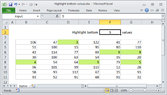
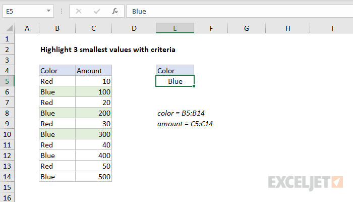
To highlight the 3 smallest values that meet specific criteria, you can use an array formula based on the AND and SMALL functions.  In the example shown, the formula used for conditional formatting is:

=AND($B5=$E$5,$C5<=SMALL(IF(color=$E$5,amount),3))

Where "color" is the named range B5:B12 and "amount" is the named range C5:C12.

How this formula works

Inside the AND function there are two logical criteria. The first is straightforward, and ensures that only cells that match the color in E5 are highlighted:

$B3=$E$5

The second test is more complex:

$C3<=SMALL(IF(color=$E$5,amount),3)

Here, we filter amounts to make sure that only values associated with the color in E5 (blue) are retained. The filtering is done with the IF function like this:

IF(color=$E$5,amount)

The resulting array looks like this:

{FALSE;100;FALSE;200;FALSE;300;FALSE;400;FALSE;500}

Notice the value from the amount column only survives if the color is "blue". Other amounts are now FALSE.

Next, this array goes into the SMALL function with a k value of 3, and SMALL returns the "3rd smallest" value, 300. The logic for the second logical test reduces to:

$C3<=300

When both logical conditions are return TRUE, the conditional formatting is triggered and cells are highlighted.

Note: this is an array formula, but does not require control + shift + enter.