Summary
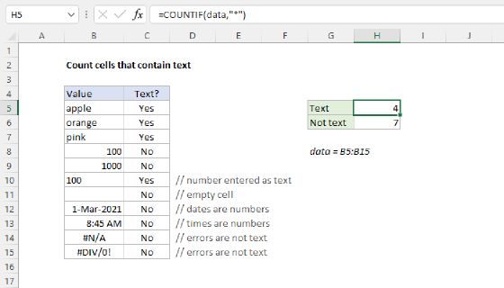
To count cells that contain certain text, you can use the COUNTIF function with a wildcard. In the example shown, the formula in E5 is:
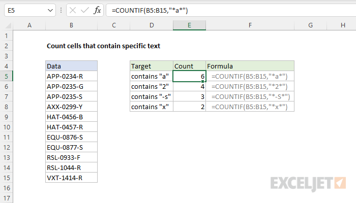
=COUNTIF(B5:B15,"*a*")
The result is 6, since there are six cells in B5:B15 that contain the letter "a".
Generic formula
=COUNTIF(range,"*txt*")
Explanation
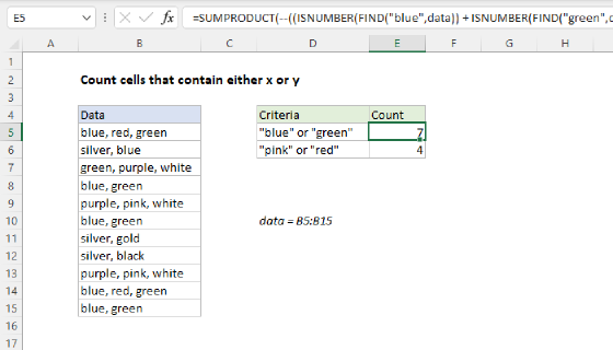
In this example, the goal is to count cells that contain a specific substring. This problem can be solved with the SUMPRODUCT function or the COUNTIF function. Both approaches are explained below. The SUMPRODUCT version can also perform a case-sensitive count.
COUNTIF function
The COUNTIF function counts cells in a range that meet supplied criteria. For example, to count the number of cells in a range that contain "apple" you can use COUNTIF like this:
=COUNTIF(range,"apple") // equal to "apple"
Notice this is an exact match. To be included in the count, a cell must contain "apple" and only "apple". If a cell contains any other characters, it will not be counted.
In the example shown, the goal is to count cells that contain specific text, meaning the text is a substring that can be anywhere in the cell. To do this, we need to use the asterisk (*) character as a wildcard. To count cells that contain the substring "apple", we can use a formula like this:
=COUNTIF(range,"*apple*")
The asterisk (*) wildcard matches zero or more characters of any kind, so this formula will count cells that contain "apple" anywhere in the cell. The formulas used in the worksheet shown follow the same pattern:
=COUNTIF(B5:B15,"*a*") // contains "a"
=COUNTIF(B5:B15,"*2*") // contains "2"
=COUNTIF(B5:B15,"*-S*") // contains "-s"
=COUNTIF(B5:B15,"*x*") // contains "x"
You can easily adjust this formula to use a cell reference in criteria. For example, if A1 contains the text you want to match, you can use:
=COUNTIF(range,"*"&A1&"*")
Inside COUNTIF, the two asterisks are concatenated to the value in A1, and the formula works as before. The COUNTIF function supports three different wildcards, see this page for more details.
Note the COUNTIF formula above won't work if you are looking for a particular number and cells contain numeric data. This is because the wildcard automatically causes COUNTIF to look for text only (i.e. to look for "2" instead of just 2). Because a text value won't ever be found in a true number, COUNTIF will return zero. In addition, COUNTIF is not case-sensitive, so you can't perform a case-sensitive count. The SUMPRODUCT alternative below can handle both cases.
SUMPRODUCT function
Another way to solve this problem is with the SUMPRODUCT function and Boolean algebra. This approach has the benefit of being case-sensitive if needed. In addition, you can use this technique to find a number inside of a number, something you can't do with COUNTIF.
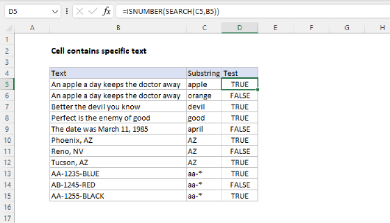
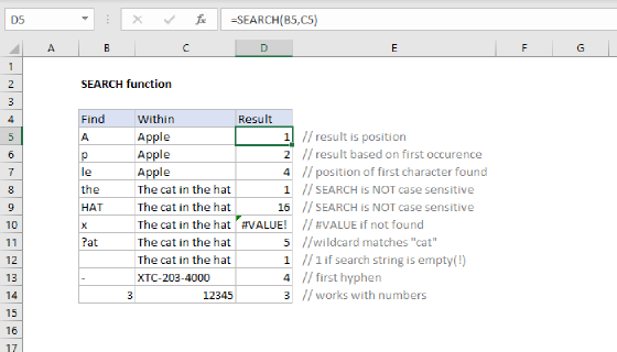
To count cells that contain specific text with SUMPRODUCT, you can use the SEARCH function. SEARCH returns the position of text in a text string as a number. For example, the formula below returns 6 since the "a" appears first as the sixth character in the string:
=SEARCH( "a","The cat sat") // returns 6
If the text is not found, SEARCH returns a #VALUE! error:
=SEARCH( "x","The cat sat") // returns #VALUE!
To count cells that contain "a" in the worksheet shown with SUMPRODUCT, you can use the ISNUMBER and SEARCH functions like this:
=SUMPRODUCT(--ISNUMBER(SEARCH("a",B5:B15)))
Working from the inside out, the logical test inside SUMPRODUCT is based on SEARCH:
SEARCH("a",B5:B15)
Because the range B5:B15 contains 11 cells, the result from SEARCH is an array with 11 results:
{1;1;1;1;2;2;#VALUE!;#VALUE!;#VALUE!;#VALUE!;#VALUE!}
In this array, numbers indicate the position of "a" in cells where "a" is found. The #VALUE! errors indicate cells where "a" was not found. To convert these results into a simple array of TRUE and FALSE values, the SEARCH function is nested in the ISNUMBER function:
ISNUMBER(SEARCH("a",B5:B15))
ISNUMBER returns TRUE for any number and FALSE for errors. SEARCH delivers the array of results to ISNUMBER, and ISNUMBER converts the results to an array that contains only TRUE and FALSE values:
{TRUE;TRUE;TRUE;TRUE;TRUE;TRUE;FALSE;FALSE;FALSE;FALSE;FALSE}
In this array, TRUE corresponds to cells that contain "a" and FALSE corresponds to cells that do not contain "a". We want to count these results, but we first need to convert the TRUE and FALSE values to their numeric equivalents, 1 and 0. To do this, we use a double negative (--):
--ISNUMBER(SEARCH("a",B5:B15))
The result inside of SUMPRODUCT looks like this:
=SUMPRODUCT({1;1;1;1;1;1;0;0;0;0;0}) // returns 6
With a single array to process, SUMPRODUCT sums the array and returns 6 as a final result.
One benefit of this formula is it will find a number inside a numeric value. In addition, there is no need to use wildcards to indicate position, because SEARCH will automatically look through all text in a cell.
Case-sensitive option
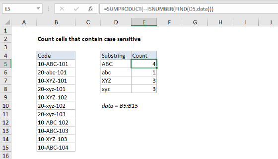
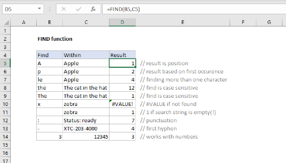
For a case-sensitive count, you can replace the SEARCH function with the FIND function like this:
=SUMPRODUCT(--(ISNUMBER(FIND(text,range))))
The FIND function works just like the SEARCH function, but is case-sensitive. You can use a formula like this to count cells that contain "APPLE" and not "apple". This example provides more detail.