Explanation
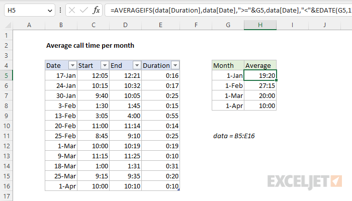
In this example, the goal is to calculate the average call time (duration in minutes) for each month listed in column G using the dates in column B and the durations in column E. The article below explains two approaches. The first formula is based on the AVERAGEIFS function, which is designed to calculate averages using multiple criteria. The second formula is based on the FILTER function and the AVERAGE function. For convenience, all data is in an Excel Table named data in the range B5:E16.
Note: the values in G5:G8 are valid Excel dates. This makes it easier to use these values in the formula criteria. You can use a custom number format to display these dates any way you like.
AVERAGEIFS function
The AVERAGEIFS function calculates the average of cells in a range that meet one or more conditions, referred to as criteria. The generic syntax for AVERAGEIFS looks like this:
=AVERAGEIFS(avg_range,range1,criteria1,range2,criteria2,...)Notice each condition is entered as a separate [range, criteria] pair. In this problem, we need to configure AVERAGEIFS to average amounts by month using two criteria: (1) dates greater than or equal to the first day of the month, (2) dates less than the first day of the next month. We start off with the average range, which is the call durations column in the table:
=AVERAGEIFS(data[Duration],Next, we need to enter the criteria needed to target the right dates for each month. To make this step easier, the values in G5:G8 are entered as "first of month" dates. For the start date, we use the data[Date] column for the criteria range and the greater than or equal to operator (>=) concatenated to cell G5 for the criteria:
=AVERAGEIFS(data[Duration],data[Date],">="&G5,For the end date, we again use the data[Date] column for the criteria range:
=AVERAGEIFS(data[Duration],data[Date],">="&G5,data[Date],For criteria, we use the EDATE function to return the first day of the next month:
=EDATE(E5,1) // first of next month
The final formula in H5, copied down, is:
=AVERAGEIFS(data[Duration],data[Date],">="&G5,data[Date],"<"&EDATE(G5,1))Notice we need to concatenate the dates to logical operators, as required by the AVERAGEIFS function. The structured references behave like absolute references and don't change, while the reference to G5 is relative and changes at each new row. As the formula is copied down, it returns an average call duration for each month in column G.
FILTER with AVERAGE
Another nice way to average by month is to use the FILTER function with the AVERAGE function like this:
=AVERAGE(FILTER(data[Duration],TEXT(data[Date],"mmyy")=TEXT(G5,"mmyy")))Working from the inside out, the FILTER function extracts the durations for a given month and returns these amounts to the AVERAGE function, which calculates an average. The FILTER function is configured like this:
FILTER(data[Duration],TEXT(data[Date],"mmyy")=TEXT(G5,"mmyy"))The first argument, array, is set to data[Duration]. The second argument, include, is where most of the work gets done:
TEXT(data[Date],"mmyy")=TEXT(G5,"mmyy")Here, we use the TEXT function to convert the dates to text strings in the format "mmyy". Because there are 12 dates in the list, all in 2023, the result is an array with 12 values like this:
{"0123";"0123";"0123";"0223";"0223";"0223";"0223";"0323";"0323";"0323";"0323";"0423"}
Next, the TEXT function is used in the same way to extract the month and year from the date in G5:
TEXT(G5,"mmyy") // returns "0123"
The two results above are then compared to each other. The result is an array of 12 TRUE and FALSE values like this:
{TRUE;TRUE;TRUE;FALSE;FALSE;FALSE;FALSE;FALSE;FALSE;FALSE;FALSE;FALSE}In this array, a TRUE value indicates dates in B5:B16 that are in the same month and year as the date in G5, i.e. January dates. The FILTER function uses this array to retrieve only values in January. The result is delivered directly to the AVERAGE function like this:
{0.0111111111111111;0.0118055555555556;0.0173611111111112}Excel times are just fractional parts of 1 day, so the decimal numbers represent time in a raw number format. AVERAGE then returns a result of approximately 0.01343, which, when formatted with the custom number format "mm:ss", displays as 19:20. As the formula is copied down, FILTER delivers durations for each month to the AVERAGE function, which returns a final result.
Note: the overall structure of this formula is more compact and elegant, so you might wonder why we don't use the TEXT function in the same way with the AVERAGEIFS function? Unfortunately, this is not possible because AVERAGEIFS won't accept an array operation in a range argument. This is a limitation of the *IFS functions in Excel, which you can read more about here.
Pivot Table solution
A pivot table is an excellent solution when you need to summarize or average data by year, month, quarter, and so on, because pivot tables provide controls for grouping dates automatically. For a side-by-side comparison of formulas vs. pivot tables, see this video: Why pivot tables.


