Average hourly pay per day

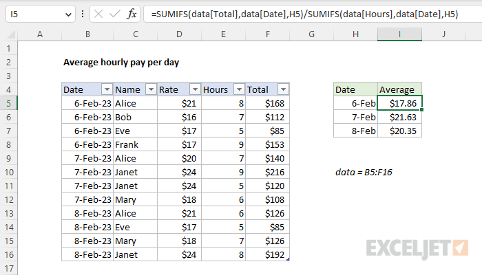
In this example, the goal is to calculate the average hourly rate per day based on the data shown. All data is in Excel Table named data in the range B5:F16. Note that we want to calculate a weighted average in this case. A weighted average hourly rate is the average rate at which the workers are paid, taking into account the number of hours worked at each rate. This weighted average is calculated by multiplying each rate by its corresponding weight (hours worked) for a given date, then dividing by the sum of the hours logged on that date. The solution shown requires four general steps:

1. Create an Excel Table called data
2. Create a summary table for results, like H4:I7 in the example
3. Enter the formula and copy it down the summary table

Create the Excel Table

One of the key features of an Excel Table is its ability to dynamically resize when rows are added or removed. In this case, all we need to do is create a new table named data with the data shown in B5:D16.  You can use the keyboard shortcut Control + T.

Video: How to create an Excel table

The table will now automatically expand or contract as needed when new data is added or removed.

Total amounts per date

Because we have the total for each entry in column F, we already have rates * hours. This means we can just use the SUMIFS function (the SUMIF function would work fine too) to get a total for each date with a formula like this:

SUMIFS(data[Total],data[Date],H5)

The sum_range is the Total column, the criteria_range is the Date column, and the criteria itself is the date in cell H5. By itself, this formula will return the total Amount for each date.

Total hours per date

The next step is to calculate the total hours per date. To do this, we can again use the SUMIFS function in a very similar formula:

SUMIFS(data[Hours],data[Date],H5)

In this formula, the sum_range is the Hours column, and the criteria_range and criteria are the same as the formula above. This formula will return the total Hours logged for each date.

Divide amounts by hours

The last step is to divide the total amount per date by the total hours per date like this:

=SUMIFS(data[Total],data[Date],H5)/SUMIFS(data[Hours],data[Date],H5)

In cell I5, the formula is solved like this:

=SUMIFS(data[Total],data[Date],H5)/SUMIFS(data[Hours],data[Date],H5)
=518/29
=17.86

SUMPRODUCT alternative

As mentioned above, because we have hours * rate already in column F as Amount, we can use this value directly in the SUMIFS formula as shown. However, in cases where the data does not contain hours * rate, you can use the SUMPRODUCT function to run this calculation inside the formula like this:

=SUMPRODUCT((data[Date]=H5)*data[Hours]*data[Rate])/SUMIFS(data[Hours],data[Date],H5)

This formula returns the same result, but does not need the Amount in column F to be part of the data. Why not do the same thing with SUMIFS? It's a bit technical, but the reason we can't take the same approach with SUMIFS is that SUMIFS is in a group of eight Excel functions that require a range. This means we can't supply a calculation for the sum range in this case.