Average numbers ignore zero

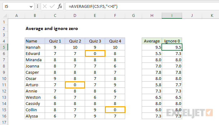
In this example, the goal is to calculate an average of the quiz scores in columns C, D, E, and F for each person. However, the result needs to ignore any zeros that appear in the data. This formula can be easily solved with the AVERAGEIF function or the AVERAGEIFS function. It can also be solved with a combination of FILTER and AVERAGE. See below for details.

AVERAGE function

The standard way to calculate an average in Excel with a formula is to use the AVERAGE function. You can see the results from AVERAGE in column H of the worksheet shown. The formula in H5, copied down, is:

=AVERAGE(C5:F5)

However, while AVERAGE will ignore text values and empty cells, it will not ignore zero values like those in cell E6, D11, and F15. An easy solution in this case is to switch to the AVERAGEIF or AVERAGEIFS function instead.

AVERAGEIF function

The AVERAGEIF function calculates the average of the numbers in a range that meet a single condition. To apply criteria, AVERAGEIF supports logical operators (>,<,<>,=) and wildcards (*,?) for partial matching. In this case, we can use AVERAGEIFS to solve this problem by excluding zero values with the criteria "<>0". The formula in cell I5, copied down, is:

=AVERAGEIF(C5:F5,"<>0")

Note that the average returned by AVERAGEIF is higher than the average calculated by AVERAGE in rows 6, 11, and 16. This is the effect of excluding Quiz scores equal to zero.

AVERAGEIFS function

The AVERAGEIFS function works like AVERAGEIF, except it is designed to apply multiple criteria. We can use AVERAGEIFS to solve this problem by excluding zero values with the criteria "<>0" like this:

=AVERAGEIFS(C5:F5,C5:F5,"<>0")

One difference between AVERAGEIFS and AVERAGEIF is that the average range is always the first argument with AVERAGEIFS, and is required. With AVERAGEIF the average range is the last argument and is optional. For more details on the syntax of AVERAGEIFS with many more examples, see this page.

AVERAGE with FILTER

Another way to solve this problem in the current version of Excel is to use the AVERAGE function together with the FILTER function in a formula like this:

=AVERAGE(FILTER(C5:F5,C5:F5<>0))

This is a newer and more flexible way to handle this problem. The FILTER function is configured to select only quiz scores that are not equal to zero like this:

=FILTER(C5:F5,C5:F5<>0)

The result from FILTER is an array that contains only non-zero quiz scores. This array is returned directly to the AVERAGE function, which calculates the average. Zero values never make it into the AVERAGE function to start with. For more on FILTER, see this page.