TRANSPOSE Function

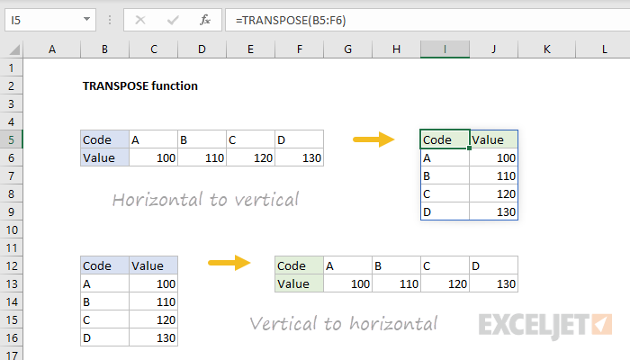
The TRANSPOSE function converts a vertical range of cells to a horizontal range of cells, or a horizontal range of cells to a vertical range of cells. In other words, TRANSPOSE "flips" the orientation of a given range or array:

1. When given a vertical range, TRANSPOSE converts it to a horizontal range
2. When given a horizontal range, TRANSPOSE converts it to a vertical range

When array is transposed, the first row becomes the first column of the new array, the second row becomes the second column of the new array, the third row becomes the third column of the new array, and so on.

TRANSPOSE can be used with both ranges and arrays. Transposed ranges are dynamic. If data in the source range changes, TRANSPOSE will immediately update data in the target range.

Examples

When given a vertical array, TRANSPOSE returns a horizontal array:

=TRANSPOSE({"a";"b";"c"}) // returns {"a","b","c"}

To transpose the vertical range A1:A5 into a horizontal array:

=TRANSPOSE(A1:A5) // vertical to horizontal

To transpose the horizontal range A1:E1 to a vertical array:

=TRANSPOSE(A1:E1) // vertical to horizontal

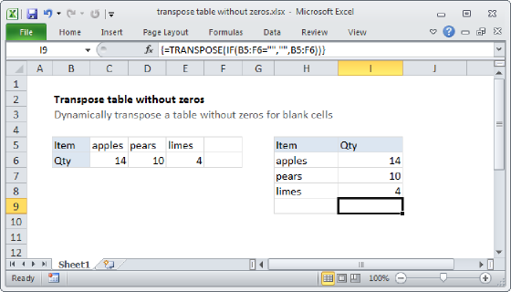
In the example shown above, the formulas in I5 and F12 are:

=TRANSPOSE(B5:F6) // formula in I5
=TRANSPOSE(B12:C16) // formula in F12

Note: TRANSPOSE does not carry over formatting. In the example shown, the target ranges have been formatted in a separate step.

TRANSPOSE with other functions

TRANSPOSE can be used to "catch" and transpose the output from another function. The formula below changes the result from XLOOKUP from a horizontal configuration to a vertical configuration:

=TRANSPOSE((XLOOKUP(value,lookup_range,return_range))

Read more: XLOOKUP wildcard example.

Excel 365

In Excel 365, which supports dynamic array formulas, no special syntax is required, TRANSPOSE simply works and results spill into destination cells automatically. However, in other versions of of Excel, TRANSPOSE must be entered as a multi-cell array formula with control + shift + enter:

1. First select the target range, which should have the same number of rows as the source range has columns, and the same number of columns as the source range has rows.
2. Enter the TRANSPOSE function, and select the source range as the array argument.
3. Confirm the formula as an array formula with control + shift + enter.

Paste special

The TRANSPOSE function makes sense when you need a dynamic solution that will continue to update when source data changes. However if you only need a one-time conversion, you can use Paste Special with the Transpose option. This video covers the basics of Paste Special.