Summary
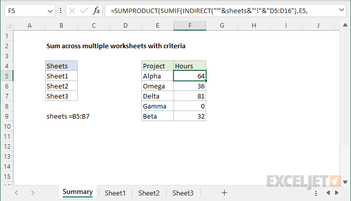
To conditionally sum identical ranges in separate worksheets, you can use a formula based on the SUMIF function, the INDIRECT function, and the SUMPRODUCT function. In the example shown, the formula in F5 is:
=SUMPRODUCT(SUMIF(INDIRECT("'"&sheets&"'!"&"D5:D16"),E5,INDIRECT("'"&sheets&"'!"&"E5:E16")))
where sheets is the named range B5:B7. As the formula is copied down, it returns total hours in Sheet1, Sheet2, and Sheet3 for the projects shown in column E.
Note: you might wonder why we don't use the SUMIF function with a 3D reference to sum multiple worksheets with criteria? The problem is that SUMIFS, COUNTIFS, AVERAGEIFS, etc. are in a group of functions that do not support 3D references.
Generic formula
=SUMPRODUCT(SUMIF(INDIRECT("'"&sheets&"'!"&"rng"),criteria,INDIRECT("'"&sheets&"'!"&"sum_rng")))
Explanation
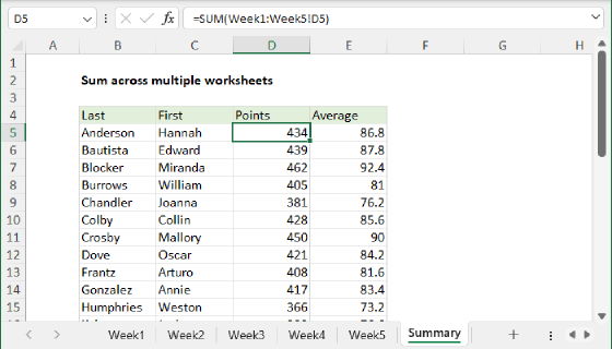
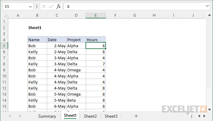
In this example, the goal is to sum hours per project across three different worksheets: Sheet1, Sheet2, and Sheet3. The data on each of the three sheets has the same structure as Sheet1, as seen below:
3D reference won't work
Before we look at a solution, let's look at something that doesn't work. You might wonder if we can provide the SUMIF function with a 3D reference like this:
Sheet1:Sheet3!D5:D16
This is the standard 3D reference syntax, but if you try to use it with SUMIF, you'll get a #VALUE error. The problem is that SUMIFS, COUNTIFS, AVERAGEIFS, etc. are in a group of functions that do not support 3D references.
Workaround with INDIRECT
To workaround this problem we can use a named range "sheets" that holds the name of each worksheet that should be included in the calculation. In the example shown, sheets is the named range B5:B7, which holds three values: "Sheet1", "Sheet2", and "Sheet3". The formula in F5 is:
=SUMPRODUCT(SUMIF(INDIRECT("'"&sheets&"'!"&"D5:D16"),E5,INDIRECT("'"&sheets&"'!"&"E5:E16")))
Notice we are concatenating the sheet names to the ranges we need to work with. Once the concatenation is performed, the formula looks like this:
=SUMPRODUCT(SUMIF(INDIRECT({"'Sheet1'!D5:D16";"'Sheet2'!D5:D16";"'Sheet3'!D5:D16"}),E5,INDIRECT({"'Sheet1'!E5:E16";"'Sheet2'!E5:E16";"'Sheet3'!E5:E16"})))
Notice we now have complete references based on the three sheet names provided in sheets (B5:B7). However, because we assembled these references with concatenation, these values are not actual cell references but are in fact text values. To coerce these values into valid cell references we use the INDIRECT function.
INDIRECT converts the text values to valid references and returns the result to the SUMIF function for the range and sum_range arguments. The value for criteria is provided by the reference to cell E5 ("Alpha"), which changes as the formula is copied down the column. Because the named range "sheets" contains three values, SUMIF actually runs three times, one for each reference. The result is an array with three results like this:
{24;20;20}
This array is returned directly to the SUMPRODUCT function:
=SUMPRODUCT({24;20;20})
With a single array to process, SUMPRODUCT sums the array and returns 64 for the Alpha project in cell F5. This number is the total number of hours logged to the Alpha project in all three worksheets. As the formula is copied down, it returns a total for each project shown in column E.
Note: In the latest version of Excel, you can use the SUM function instead of the SUMPRODUCT function with the same result. In Legacy Excel, SUMPRODUCT is used frequently because it can handle arrays natively without requiring Ctrl-Shift-Enter.