Summary
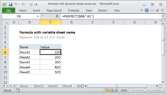
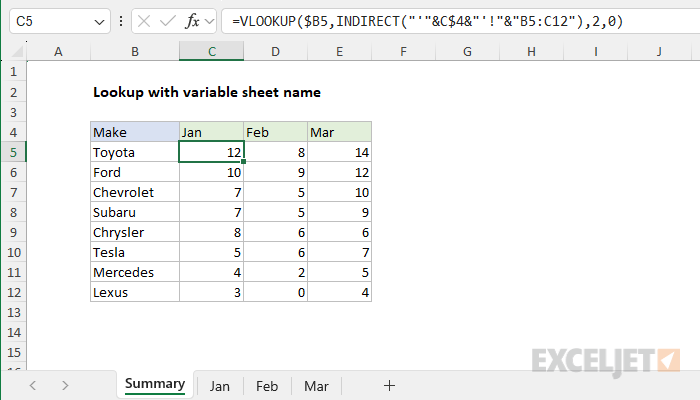
To create a lookup with a variable sheet name, you can use the VLOOKUP function together with the INDIRECT function. In the example shown, the formula in C5 is:
=VLOOKUP($B5,INDIRECT("'"&C$4&"'!"&"B5:C12"),2,0)
As the formula is copied down and across, it looks up the make in column B on each of the three worksheets (Jan, Feb, and Mar) and returns the value for that month.
Generic formula
=VLOOKUP(val,INDIRECT("'"&sheet&"'!"&"range"),col,0)
Explanation
In this example, the goal is to create a lookup formula with a variable sheet name. In other words, a formula that uses a sheet name typed into a cell to construct a reference to a range on that sheet. If the sheet name is changed, the reference should update automatically. The key to the solution explained below is the INDIRECT function which is designed to evaluate text as a worksheet reference. When the evaluation succeeds, INDIRECT converts the text into a valid reference. This makes it possible to build a formula to assemble a reference as text using concatenation, and use the resulting text as a valid reference.
Workbook setup
The workbook contains four worksheets:
- Summary - the sheet that looks up data on the other sheets
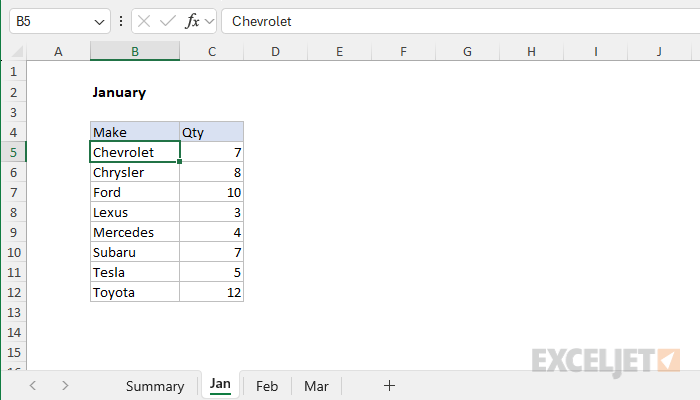
- Jan - data for January
- Feb - data for February
- Mar - data for March
Each of the monthly sheets has the same structure, which looks like this:
VLOOKUP solution
The formulas on the summary tab lookup and extract data from the month tabs, by creating a dynamic reference to the sheet name for each month, where the names for each sheet are the month names in row 4. The VLOOKUP function is used to perform the lookup. The formula in cell C5 is:
=VLOOKUP($B5,INDIRECT("'"&C$4&"'!"&"B5:C12"),2,0)
Inside VLOOKUP, the lookup value is entered as the mixed reference $B5, with the column locked to allow copying across the table. The table array is created using the INDIRECT function like this:
INDIRECT("'"&C$4&"'!"&"B5:C12")
The mixed reference C$4 refers to the column headings in row 4, which match sheet names in the workbook (i.e. "Jan", "Feb", "Mar"). A single quote character is joined to either side of C$4 using the concatenation operator (&).
The single quotes are not required in this particular example, but they allow the formula to handle sheet names that contain spaces in other workbooks.
Next, the exclamation point (!) is joined on the right to create a proper sheet reference, which is followed by the range to use as the table array. Note that the result of this concatenation is text. Next, the INDIRECT function evaluates the text and converts it to a proper reference:
=VLOOKUP($B5,INDIRECT("'"&C$4&"'!"&"B5:C12"),2,0)
=VLOOKUP($B5,INDIRECT("'Jan'!B5:C12"),2,0)
=VLOOKUP($B5,Jan!B5:C12,2,0)
Finally, VLOOKUP can finish the job. Since the data we want to retrieve is in the second column, the column index number is provided as 2. We provide zero (0) for range_lookup to force an exact match. As the formula is copied down and across, VLOOKUP retrieves the correct values from each sheet.
Notice that the sort order on the summary page is different from the sort order used on each data sheet. However, because we are using a lookup operation to retrieve the monthly values, this does not matter. VLOOKUP correctly finds and retrieves the monthly values for each make on each data sheet regardless of the order in which they appear.