Summary
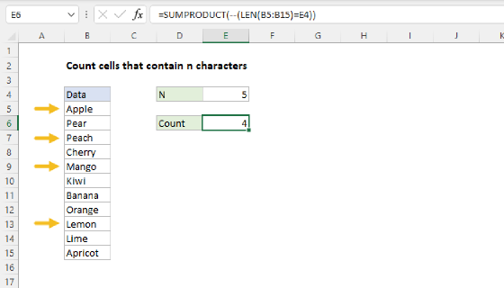
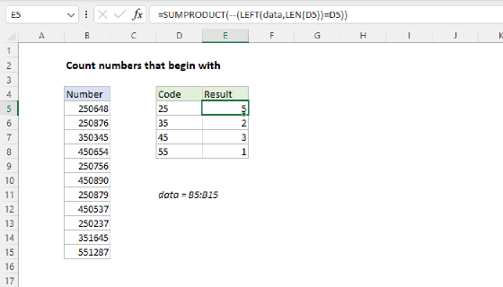
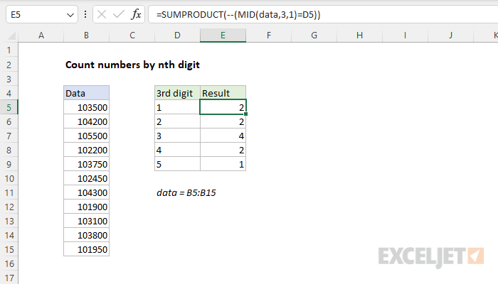
To count numbers where the nth digit is a specific number, you can use a formula based on the SUMPRODUCT function. In the example shown, the formula in E5 is:
=SUMPRODUCT(--(MID(data,3,1)=D5))
where data is the named range B5:B15 and the numbers in column D are entered as text values.
Generic formula
=SUMPRODUCT(--(MID(range,n,1)="x"))
Explanation
In this example, the goal is to count numbers in the range B5:B15 (named data) where the third digit is a specific number, indicated in column D. You might think the COUNTIF function would be a good way to solve this problem. However, for reasons explained below, COUNTIF won't work. Instead, you can use the SUMPRODUCT and Boolean logic. See below for a full explanation.
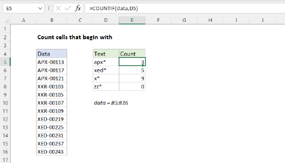
COUNTIF function
The COUNTIF function returns the count of cells that meet one or more criteria, and supports logical operators (>,<,<>,=) and wildcards (,?) for partial matching. You would think you could use the COUNTIF function with the question mark (?) and asterisk () wildcards to count numbers where the third digit is 1 like this:
=COUNTIF(data,"??1*") // returns 0
However, COUNTIF will return zero. The problem is that using any wildcard in criteria means that COUNTIF will interpret the pattern as a text value, whereas the values in column B are numeric. As a result, COUNTIF will never find a matching number and the result will always be zero. As a workaround, you might try the trick below to coerce the numbers in data to text by concatenating an empty string ("") to the range like this:
=COUNTIF(data&"","???1") // throws error
However, this will cause Excel to throw the generic "There's a problem with this formula" error, so it's not possible to even enter the formula. This happens because COUNTIF is in a group of eight functions that require an actual range for range arguments. This means you can't use an array operation to modify the range argument inside COUNTIF, COUNTIFS, SUMIF, SUMIFS, etc.
SUMPRODUCT function
Another way to solve this problem is with the SUMPRODUCT function, the MID function, and Boolean logic. To count numbers in data where the third digit is 1, we can use SUMPRODUCT like this:
=SUMPRODUCT(--(MID(data,3,1)="1")) // returns 2
Working from the inside out, the MID function is used to extract and test the third digit from the numbers in data like this:
MID(data,3,1)="1"
Because we give MID 11 numbers in the range B5:B15, MID returns an array with 11 results:
{"3";"4";"5";"2";"3";"2";"4";"1";"3";"3";"1"}="25"
Note that MID automatically converts the numbers to text, so we use the text value "1" for the comparison. The result is an array of TRUE and FALSE values:
{FALSE;FALSE;FALSE;FALSE;FALSE;FALSE;FALSE;TRUE;FALSE;FALSE;TRUE}
In this array, TRUE values correspond to numbers where the third digit is 3. We want to count these results, but first we need to convert the TRUE and FALSE values to 1s and 0s. To do this, we use a double negative (--).
--{FALSE;FALSE;FALSE;FALSE;FALSE;FALSE;FALSE;TRUE;FALSE;FALSE;TRUE}
The resulting array contains only 1s and 0s and is delivered directly to the SUMPRODUCT function:
=SUMPRODUCT({0;0;0;0;0;0;0;1;0;0;1})
With only a single array to process, SUMPRODUCT sums the items in the array and returns 2 as result. In this formula, note we are hardcoding the value "1" and we set num_chars to 1 inside the MID function. To adapt the formula for the worksheet shown, we a reference to cell D5 like this:
=SUMPRODUCT(--(MID(data,3,1)=D5))
As the formula is copied down, it returns the count of numbers in data where the third digit equals the numbers in column D. Note that the numbers in column D are entered as text values, since the result from MID will also be text. You can avoid this requirement by adapting the formula to coerce the value in D5 to text:
=SUMPRODUCT(--(MID(data,3,1)=D5&""))
Here we concatenate an empty string ("") to the D5, which will convert a numeric value to text. This version of the formula will work when there are numbers in column D, or text values.
Note: In Excel 365 and Excel 2021 you can use the SUM function instead of SUMPRODUCT if you prefer. This article provides more detail.