Summary
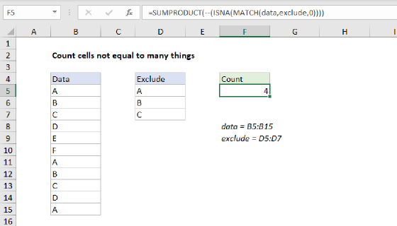
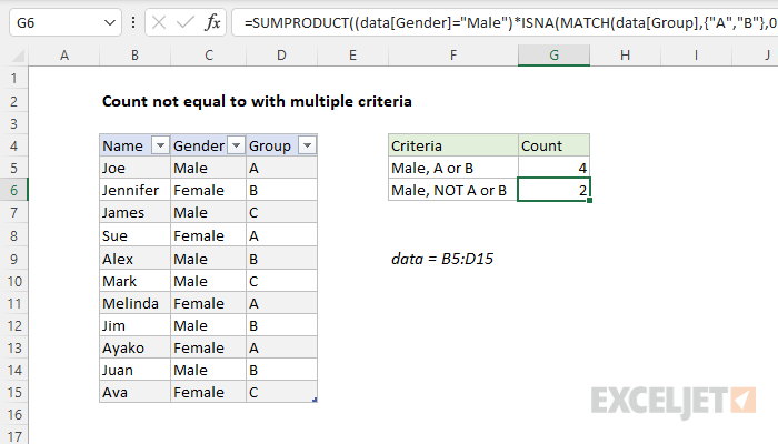
To count rows not equal to multiple criteria, you can use the SUMPRODUCT function together with the MATCH and ISNA functions. In the example shown, the formula in G6 is:
=SUMPRODUCT((data[Gender]="Male")*ISNA(MATCH(data[Group],{"A","B"},0)))
Where data is an Excel Table in the range B5:D15. The result is 2 since two males are not in Group A or B.
Note: You can also solve this problem with the COUNTIFS function, as explained below. The SUMPRODUCT formula is more advanced, but it scales better when there are many exclusions.
Generic formula
=SUMPRODUCT((range=criteria)*ISNA(MATCH(range,criteria,0)))
Explanation
In this example, the goal is to count rows in a set of data using multiple criteria and "not equals to" logic. Specifically, we want to count males that are not in group A or B. All data is in an Excel Table named data in the range B5:D15. This problem can be solved with the COUNTIFS function or the SUMPRODUCT function. Both approaches are explained below.
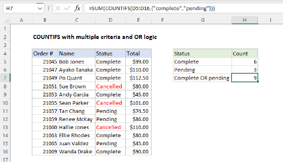
COUNTIFS function
The COUNTIFS function returns the count of cells that meet one or more criteria, and supports logical operators (>,<,<>,=) and wildcards (*,?) for partial matching. Conditions are supplied to COUNTIFS in the form of range/criteria pairs — each pair contains one range and the associated criteria for that range:
=COUNTIFS(range1,criteria1,range2,criteria2,etc)
In this case, the first condition is that Gender is Male:
=COUNTIFS(data[Gender],"Male") // returns 6
The result is 6, since there are six Males in the table. Next, we need to exclude group "A":
=COUNTIFS(data[Gender],"Male",data[Group],"<>A")
This formula returns 5. Notice we use the not equal to operator (<>) enclosed in double quotes. Finally, we need to exclude group B with another range/criteria pair:
=COUNTIFS(data[Gender],"Male",data[Group],"<>A",data[Group],"<>B")
Notice the syntax to exclude group B is the same and both conditions use the same range. This formula returns 2. The COUNTIFS function joins all criteria with AND logic, so it works well to exclude A and B in this case. As more exclusions are added however, the syntax gets more cumbersome, because each new exclusion requires another range/criteria pair. The SUMPRODUCT option below scales more easily.
SUMPRODUCT function
Another way to solve this problem is with the SUMPRODUCT function and Boolean logic. To start off, we can count males like this:
=SUMPRODUCT(--(data[Gender]="Male")) // returns 6
Working from the inside out, this expression tests all values in the Gender column for "Male":
data[Gender]="Male"
Since there are 11 cells in the column, the result is an array with 11 TRUE and FALSE values:
{TRUE;FALSE;TRUE;FALSE;TRUE;TRUE;FALSE;TRUE;FALSE;TRUE;FALSE}
Each TRUE represents a "Male" in the Gender column. SUMPRODUCT will ignore TRUE and FALSE values by default, so we need to convert these TRUE and FALSE values to their numeric equivalents, 1 and 0. A simple way to do this is with a double negative (--):
--(data[Gender]="Male")
The result from this snippet is an array like this:
{1;0;1;0;1;1;0;1;0;1;0}
Notice the TRUE values are now 1s. This array is delivered to SUMPRODUCT, which returns 6:
=SUMPRODUCT({1;0;1;0;1;1;0;1;0;1;0}) // returns 6
Next, we need to exclude groups "A" and "B". A good way to do this is with the MATCH function together with the ISNA function like this:
ISNA(MATCH(data[Group],{"A","B"},0))
Notice the configuration of MATCH is "reversed". The lookup_value is given as data[Group], and the lookup_array is given as the array constant {"A","B"}. We do it this way to keep the rows in the output array consistent with the table. The result from MATCH is an array like this:
{1;2;#N/A;1;2;#N/A;1;2;1;2;#N/A}
This array has 11 rows, like the data table. The numbers indicated rows where group "A" or "B" were found. The #N/A errors indicate rows where group "A" or "B" were not found. To convert this array into something we can use, we use the ISNA function:
ISNA(MATCH(data[Group],{"A","B"},0))
The result from ISNA is an array of TRUE and FALSE values like this:
{FALSE;FALSE;TRUE;FALSE;FALSE;TRUE;FALSE;FALSE;FALSE;FALSE;TRUE}
ISNA returns TRUE only for the #N/A errors, so the TRUE values in this array indicate rows where the group was not "A" or "B". If we wanted to use this expression in SUMPRODUCT by itself, we would use a formula like this:
=SUMPRODUCT(--ISNA(MATCH(data[Group],{"A","B"},0)))
The double negative (--) again converts TRUE and FALSE values, and the result looks like this:
=SUMPRODUCT({0;0;1;0;0;1;0;0;0;0;1}) // returns 3
The result is 3, since there are 3 records not in group A or B.
Putting it all together
The next step is to put both tests above together inside SUMPRODUCT like this:
=SUMPRODUCT((data[Gender]="Male")*ISNA(MATCH(data[Group],{"A","B"},0)))
Notice we use multiplication (*) to join the two expressions. We do this because multiplication corresponds to AND logic in Boolean algebra. Also notice that we no longer need the double negative (--). This is because the math operation of multiplication automatically converts the TRUE and FALSE values to 1s and 0s. The formula evaluates like this:
=SUMPRODUCT({1;0;1;0;1;1;0;1;0;1;0}*{0;0;1;0;0;1;0;0;0;0;1})
=SUMPRODUCT({0;0;1;0;0;1;0;0;0;0;0})
=2
The final result is 2 since two males are not in Group A or B.
Note: In Excel 365 and Excel 2021 you can use the SUM function instead of SUMPRODUCT if you prefer. This article provides more detail.