Summary
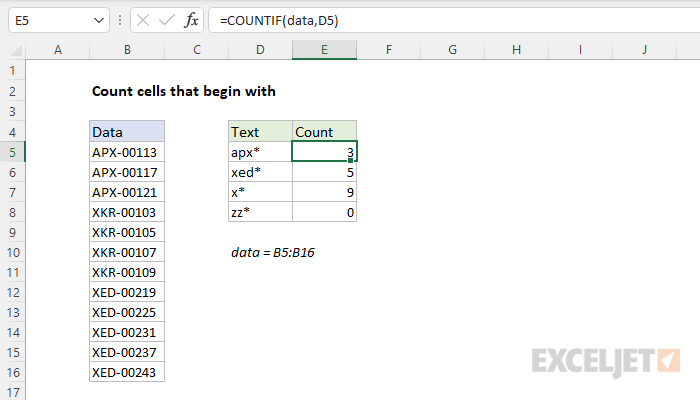
To count the number of cells that begin with specific text, you can use the COUNTIF function with a wildcard. In the example shown, the formula in cell E5 is:
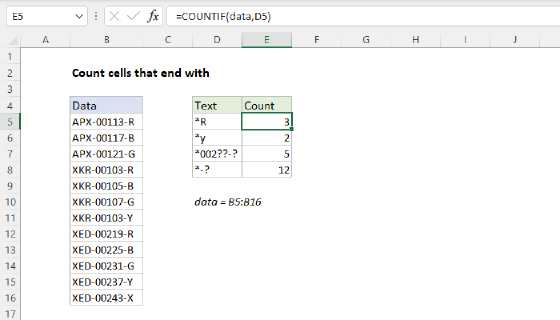
=COUNTIF(data,D5)
where data is the named range B5:B16. COUNTIF returns 3, since there are three cells that begin with "apx". Note that COUNTIF is not case-sensitive. See below for a case-sensitive formula.
Generic formula
=COUNTIF(range,"text*")
Explanation
In this example, the goal is to count cells in the range B5:B16 that begin with specific text, which is provided in column D. For convenience, the range B5:B16 is named data.
COUNTIF function
The simplest way to solve this problem is with the COUNTIF function and a wildcard. COUNTIF supports three wildcards that can be used in the criteria argument: question mark (?), asterisk(), or tilde (~). A question mark (?) matches any one character and an asterisk () matches zero or more characters of any kind. The tilde (~) is an escape character to match literal wildcards that may appear in data. In this example, we only need to use an asterisk (*).
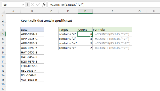
To count cells in a range that contain "apple" anywhere, you can use a formula like this:
=COUNTIF(range,"*apple*") // contain "apple" anywhere
To count cells in a range that begin with "apple" you can use a formula like this:
=COUNTIF(range,"apple*") // begin with "apple"
In the worksheet shown, we use the criteria in column D directly like this:
=COUNTIF(data,D5)
As the formula is copied down, COUNTIF returns the count of cells in data (B5:B16) that begin with the text seen in D5:D8, which already includes a wildcard. Notice that COUNTIF is not case-sensitive. The text in D5:D8 is all lowercase, yet COUNTIFS happily matches the uppercase text in B5:B16.
SUMPRODUCT function
Another way to solve this problem is to use the SUMPRODUCT function like this:
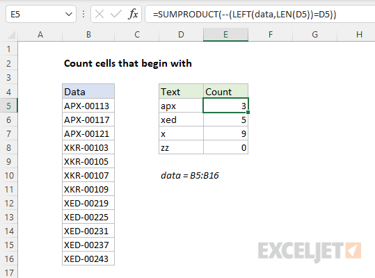
=SUMPRODUCT(--(LEFT(data,LEN(D5))=D5))
Working from the inside out, the LEFT and LEN functions are used to extract the first few characters of each value in data:
LEFT(data,LEN(D5))
Since the text in D5 is "apx", LEN returns 3, and LEFT returns the first 3 letters of all values in data in an array like this:
{"APX";"APX";"APX";"XKR";"XKR";"XKR";"XKR";"XED";"XED";"XED";"XED";"XED"}
Next, the result from LEFT is compared to the original value in D5. Since Excel is not case-sensitive by default, the result is an array of 12 TRUE and FALSE values like this:
{TRUE;TRUE;TRUE;FALSE;FALSE;FALSE;FALSE;FALSE;FALSE;FALSE;FALSE;FALSE}
Notice the TRUE values correspond to cells in data that begin with "apx".
Next, the double negative (--) converts the TRUE and FALSE values to 1s and 0s, and SUMPRODUCT sums the array and returns the result:
=SUMPRODUCT({1;1;1;0;0;0;0;0;0;0;0;0}) // returns 3
The final result is 3, since there are three values in B5:B16 that begin with "apx".
Case-sensitive option
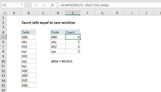
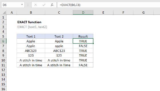
Although the SUMPRODUCT formula is more complicated than the COUNTIF formula, the nice thing about using SUMPRODUCT is that we can easily include other functions if needed. For example, to make the formula case-sensitive, we can add the EXACT function. EXACT compares values like this:
=EXACT("apple","apple") // returns TRUE
=EXACT("apple","Apple") // returns FALSE
EXACT only returns TRUE when the two text strings have exactly the same case. We can use EXACT in the formula like this:
=SUMPRODUCT(--EXACT(LEFT(data,LEN(D5)),D5))
This version of the formula uses the LEFT and LEN functions in the same way as the original formula above. The difference is that the EXACT function compares extracted text with the text in column D. Since EXACT is case-sensitive, the entire formula becomes case-sensitive:
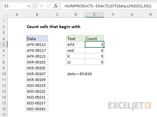
Notice the value in D6 remains lowercase, and the formula in E6 returns 0 as a result.
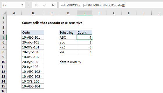
SUMPRODUCT with FIND
In Excel, there is always another way to skin the cat :) Here is another case-sensitive formula based on the FIND function:
=SUMPRODUCT(--(IFERROR(FIND(D5,data,1),0)=1))
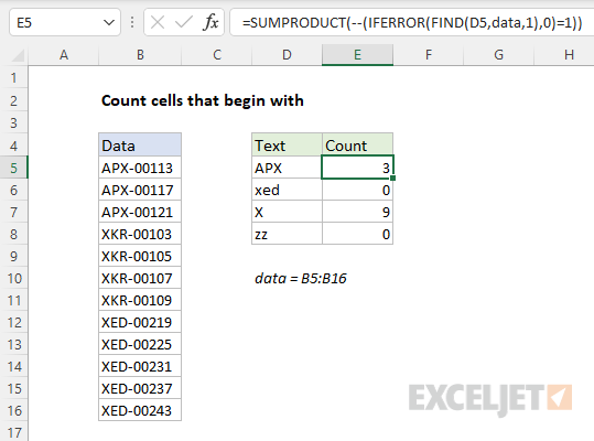
This is arguably the most elegant option, since we don't need the LEN function, the LEFT function, or the EXACT function at all. Because the FIND function is case-sensitive, we can configure FIND to look for the text in column D, and check if the result is 1, since 1 means the text was found starting at the first character.
However, one quirk of the FIND function is that it will return a #VALUE! error if the search text is not found, and this error will bubble up to the top and ruin our formula if we don't trap it. As a consequence, we have to involve the IFERROR function, just to catch the error and return 0 when it occurs. This makes the formula a bit more cryptic. Still, I do like this formula.