Sum by month in columns

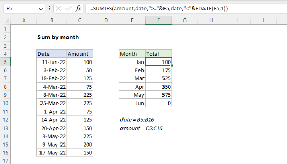
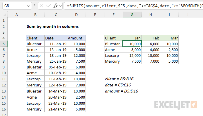
To sum by month in columns you can use the SUMIFS function together with the EOMONTH function. In the example shown, the formula in G5 is:

=SUMIFS(amount,client,$F5,date,">="&G$4,date,"<="&EOMONTH(G$4,0))

where amount (D5:D16), client (B5:B16), and date (C5:C16) are named ranges.

Explanation

In this example, the goal is to construct a formula that will subtotal the amounts in column D by client and month as seen in the range G5:I8. A big part of the problem is to set up the proper references so that the formula can be entered once, and copied throughout G5:I8. The solution explained below is based on the SUMIFS function.

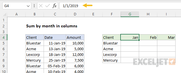
Summary table setup

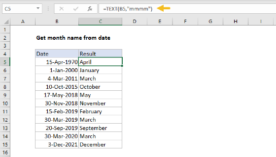
The first step in solving this problem is creating the summary table seen in the range F4:I8. The values in F4:F9 are text values. However, the month names in G4:I5 are actually valid Excel dates, formatted with the custom number format "mmm":

The month names in the summary table are actually dates

SUMIFS solution

The SUMIFS function can sum values in ranges based on multiple criteria. Multiple criteria are entered in range/criteria pairs like this:

=SUMIFS(sum_range,range1,criteria1,range2,criteria2,...)

To sum amounts by client and month with SUMIFS, we will need to enter three criteria

Client = client in column F
Date >= first of month (from date in row 4)
Date <= end of month (from date in row 4)

The first step in configuring SUMIFS is to enter the sum_range, which contains the values to sum in column D. For sum_range, we use the named range amount:

=SUMIFS(amount

Next, we need to enter the first range/criteria pair to target values in column B:

=SUMIFS(amount,client,$F5

Notice F5 is a mixed reference, with the column locked and the row relative. This allows the row to change as the formula is copied down the table, but the client name in column F does not change as the formula is copied to the right.

Next, we need to enter the second range/criteria pair, which is used to target dates that are greater than or equal to the month in G4. For the range, we use the named range date. For criteria, we use the greater than or equal to (>=) operator concatenated to the value in G4:

=SUMIFS(amount,client,$F5,date,">="&G$4

Notice G$4 this is another mixed reference, this time with the row locked. This allows the column to change as the formula is copied across the table, but keeps the row number fixed as the formula is copied down. The concatenation with an ampersand (&) is necessary when building criteria that use a logical operator and a value from another cell, because the SUMIFS function is in a group of eight functions that split criteria into two parts.

Finally, we need to enter the third range/criteria pair to check dates against the last day of the month. For the range, we again use the named range date. For criteria, we use the less than or equal to (<=) operator concatenated to the EOMONTH function:

=SUMIFS(amount,client,$F5,date,">="&G$4,date,"<="&EOMONTH(G$4,0))

We use the EOMONTH function to get the last day of the month of the date in G4. As before, we need to concatenate the result from EOMONTH to the logical operator. Again, the reference to G$4 is mixed to keep the row from changing.

As the formula is copied into the range G5:I8, the SUMIFS function returns a sum for each client and month.

Pivot Table solution

A pivot table would be an excellent solution for this problem, because it can automatically group by month without any formulas at all. For a side-by-side comparison of formulas vs. pivot tables, see this video: Why pivot tables.