Summary
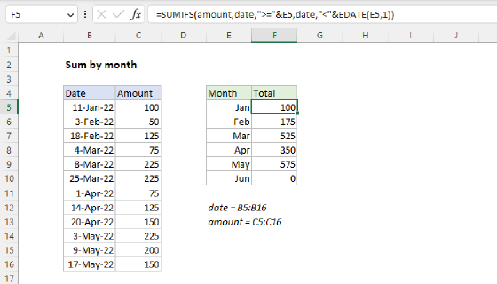
To sum data by month while ignoring year values you can use a formula based on the SUMPRODUCT function and the MONTH function. In the example shown, the formula in F5 is:
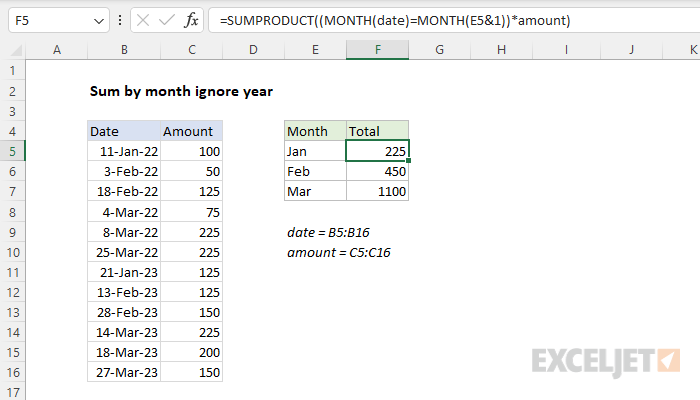
=SUMPRODUCT((MONTH(date)=MONTH(E5&1))*amount)
where amount (C5:C16) and date (B5:B16) are named ranges. The result in F5 is 225, the sum of amounts in January for both 2022 and 2023. As the formula is copied down, we get a sum of amount by month that ignores years.
Generic formula
=SUMPRODUCT((MONTH(date)=number)*amount)
Explanation
In this example, the goal is to sum numeric values by month while ignoring the year that contains the date. The solution below is based on the SUMPRODUCT function, the MONTH function, and Boolean algebra. For convenience, amount (C5:C16) and date (B5:B16) are named ranges.
Basic concept
The basic concept in this formula is to extract just the month number from all dates and test this number against the month number of interest. For example, to extract the month number of the dates in date, we can use the MONTH function like this:
MONTH(date)
Because the named range date contains 12 dates, the result from MONTH is an array with 12 numbers like this:
{1;2;2;3;3;3;1;2;2;3;3;3}
These twelve numbers correspond to the month numbers of the dates seen in column B. If we want to test these numbers for dates in January (which is the first month in the year), we can write a formula like this:
=MONTH(date)=1
This formula returns an array with 12 TRUE and FALSE values like this:
{TRUE;FALSE;FALSE;FALSE;FALSE;FALSE;TRUE;FALSE;FALSE;FALSE;FALSE;FALSE}
Notice there are two TRUE values in this array, which correspond to the two dates that occur in January: one in 2022 and one in 2023. All remaining values are FALSE, since other dates do not occur in January.
To use this array of Boolean values to sum amounts in January, we can write a formula like this:
=SUMPRODUCT((MONTH(date)=1)*amount)
After the first expression runs, we have the array of TRUE and FALSE values we looked at above:
=SUMPRODUCT({TRUE;FALSE;FALSE;FALSE;FALSE;FALSE;TRUE;FALSE;FALSE;FALSE;FALSE;FALSE}*amount)
Next, the math operation of multiplying the two arrays together automatically coerces the TRUE and FALSE values into 1s and 0s, which we can visualize like this:
=SUMPRODUCT({1;0;0;0;0;0;1;0;0;0;0;0}*amount)
Now you can see how the logic works. When the two arrays are multiplied together, the 1s return the corresponding value in amount, while the 0s "cancel out" the other amounts. We are left with a single array in SUMPRODUCT like this:
=SUMPRODUCT({100;0;0;0;0;0;125;0;0;0;0;0})
With just one array to process, SUMPRODUCT sums the array and returns 225 as the final result for January. By altering the month number, we can do the same thing for other months:
=SUMPRODUCT((MONTH(date)=1)*amount) // January
=SUMPRODUCT((MONTH(date)=2)*amount) // February
=SUMPRODUCT((MONTH(date)=3)*amount) // March
In each case, the year values of the dates being tested are completely ignored.
Dynamic month
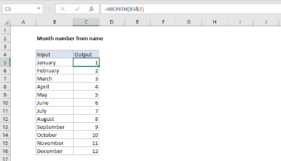
As seen above, we can hardcode month numbers into the formula and get correct results, but how can we make the formula dynamic, so that it will automatically apply the correct month number for each month seen in column F? In the worksheet, the values in F5:F7 are simply text values like "Jan", "Feb", and "Mar". One way to get a month number from a month name is to concatenate the month name to the number 1, and feed the result into MONTH like this:
=MONTH(E5&1) // returns 1
The result inside of MONTH is the string "Jan1", which Excel interprets as the date January 1 of the current year, and MONTH returns 1. We can do the same thing with E6 and E7:
=MONTH(E6&1) // returns 2
=MONTH(E7&1) // returns 3
For a more detailed explanation, see this example.
Putting it all together
The last step is to combine the ideas above into one formula:
=SUMPRODUCT((MONTH(date)=MONTH(E5&1))*amount)
This is the formula in F5 of the worksheet shown. As the formula is copied down, the month changes at each new row, and SUMPRODUCT calculates the sum of amounts for each month, ignoring year values.
Count by month ignoring year
Using the same ideas explained above, you can get a count by month like this:
=SUMPRODUCT(--(MONTH(date)=MONTH(E5&1)))
In this formula, we use a double negative (--) is used to coerce TRUE and FALSE values to 1s and 0s. This step is necessary because we don't have a math operation doing this conversion automatically.