Summary
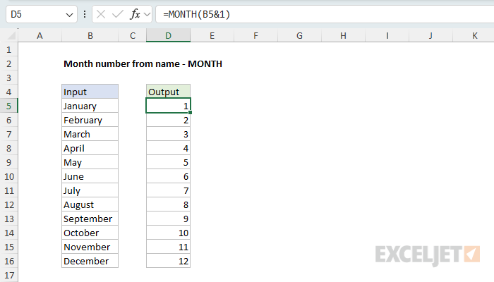
To get a standard month number from a month name (i.e. 1 from "January", 2 from "February", 3 from "March", etc.) you can use the MONTH function and a bit of concatenation. In the example shown, the formula in cell D5 is:
=MONTH(B5&1)
As the formula is copied down the column, it returns the correct number for each month. This trick depends on Excel recognizing the text as a month name, so the names must match the language of your regional settings. See below for formulas based on the XMATCH function that look up the name in a list of month names instead.
Generic formula
=MONTH(name&1)
Explanation
In this example, the goal is to return a number, 1-12, for any month name of the year. For example, given the string "January" we want to return 1, "February" should return 2, and so on. If we had a valid Excel date, we could use a number format for this task, but because we are starting with a text string, we need another way. This article explains two approaches: a classic trick that uses the MONTH function to convert the name to a date, and a more robust approach that looks up the name in a list of month names with the XMATCH function.
Table of contents
- MONTH with concatenation
- Date evaluation
- Which month names work?
- XMATCH with a list of month names
- XMATCH with generated month names
MONTH with concatenation
The approach in the example shown is to create a date fragment that can be correctly interpreted by Excel as a valid date. The formula in cell D5 is:
=MONTH(B5&1) // returns 1
Working from the inside out, we start by concatenating the name in cell B5 to the number 1:
B5&1 // returns "January1"
This expression returns a string like "January1", "February1", "March1", and so on. It turns out that if we pass a date fragment like this into the MONTH function, it will coerce the string to a valid date, using the current year. For "January1", the result is January 1 of the current year.
After this date has been created, the MONTH function returns the correct month number for the date that was created using concatenation. In each case, the actual date value is a "throwaway", used only as a convenient value to pass into the MONTH function, so the year doesn't matter. In D5 the evaluation works like this:
=MONTH(B5&1)
=MONTH("January1") // January 1 of the current year
=1
Date evaluation
This example is a bit tricky in that the evaluation of the date inside the MONTH function is automatic. If you use the expression that concatenates the month name to 1 outside the MONTH function, you'll need to add an extra step to get Excel to convert the text to a date. The DATEVALUE function or adding zero are both good options:
=DATEVALUE(B5&1)
=(B5&1)+0
Both will return a date serial number, which must then be formatted as a date. Both also ask Excel to convert text to a date, so the month-name rules below apply to them too.
Which month names work?
Because this formula asks Excel to convert text to a date, it only works when Excel recognizes the text as a month name. Full names and three-letter abbreviations work, and case doesn't matter. Excel will even accept a name shortened to three or more letters, like "Sept". But an abbreviation with a period fails, and so does a name with a leading space:
=MONTH("January"&1) // returns 1
=MONTH("JAN"&1) // returns 1
=MONTH("Sept"&1) // returns 9
=MONTH("Jan."&1) // returns #VALUE!
=MONTH(" June"&1) // returns #VALUE!
The bigger catch is language. Excel reads the month name using your computer's regional settings, so the names must be in that language. With English settings, "Juni" (German) and "Enero" (Spanish) both return #VALUE!. "Januar" (German) works, but only because it happens to match the first six letters of "January". If you can't be sure Excel will recognize the month names in your data, use one of the XMATCH formulas below, which look up the name in a list instead of converting it to a date.
XMATCH with a list of month names
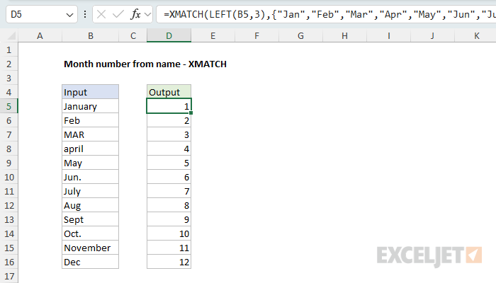
A more robust way to solve this problem is to look up the month name in a list of the 12 month names. The position of the name in the list is the month number. In the worksheet below, the month names are entered in several different formats, and the formula in D5 is:
=XMATCH(LEFT(B5,3),{"Jan","Feb","Mar","Apr","May","Jun","Jul","Aug","Sep","Oct","Nov","Dec"})
Working from the inside out, the LEFT function extracts the first three characters of the name in B5:
LEFT(B5,3) // returns "Jan"
The list of month names is an array constant that holds the 12 three-letter abbreviations in order. XMATCH looks for "Jan" in this array and returns its position:
=XMATCH("Jan",{"Jan","Feb","Mar","Apr","May","Jun","Jul","Aug","Sep","Oct","Nov","Dec"}) // returns 1
XMATCH performs an exact match by default, and it is not case-sensitive, so "jan" and "JAN" match too. Because only the first three characters are compared, full names ("January"), abbreviations ("Jan"), and abbreviations with a period ("Jan.") all work. And because this formula doesn't ask Excel to interpret a date, it returns the same result on any computer. In the worksheet above, MONTH(B5&1) would return #VALUE! for "Jun." and "Oct.", but XMATCH handles them without trouble.
If your month names are in another language, type those names into the array constant. If two months share the same first three letters (juin and juillet in French), remove LEFT and list the full month names instead.
XMATCH is available in Excel 2021+ and Excel 365. In older versions of Excel, you can use the MATCH function with match_type set to zero for an exact match:
=MATCH(LEFT(B5,3),{"Jan","Feb","Mar","Apr","May","Jun","Jul","Aug","Sep","Oct","Nov","Dec"},0)
XMATCH with generated month names
If you would rather not type the month names, you can generate them with the TEXT function, the DATE function, and the SEQUENCE function. In the worksheet below, the formula in D5 is:
=XMATCH(LEFT(B5,3),TEXT(DATE(2000,SEQUENCE(12),1),"mmm"))
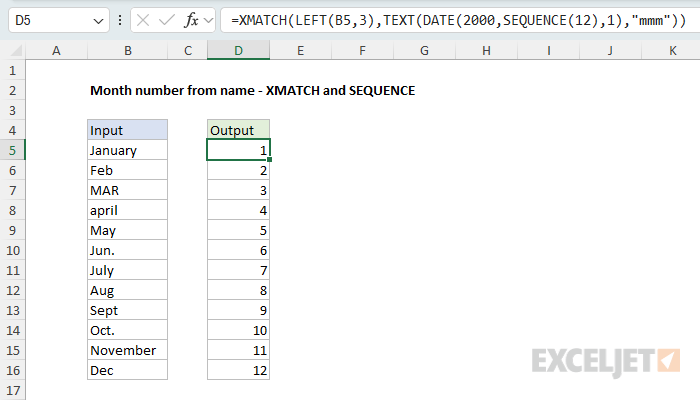
Working from the inside out, SEQUENCE(12) returns the numbers 1 to 12 in an array, and DATE uses these numbers as months to create 12 dates, the first day of each month in the year 2000 (any year will do). TEXT then converts each date to a three-letter month name with the number format "mmm":
{"Jan";"Feb";"Mar";"Apr";"May";"Jun";"Jul";"Aug";"Sep";"Oct";"Nov";"Dec"}
This array is delivered to XMATCH as the lookup array, and the formula works as before. One difference to be aware of: TEXT returns month names in the language of your regional settings. The array above is the result with English settings. With other settings the names change, so like the MONTH formula, this version depends on the computer it runs on. If the workbook needs to behave the same everywhere, use the array constant above.