Summary
Note: Excel contains many built-in "presets" for highlighting values above / below / between / equal to certain values, but if you want more flexibility you can apply conditional formatting using your own formula as explained in this article.
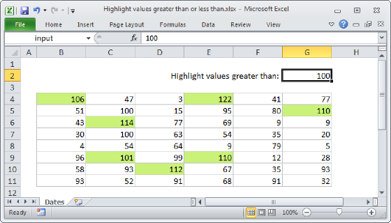
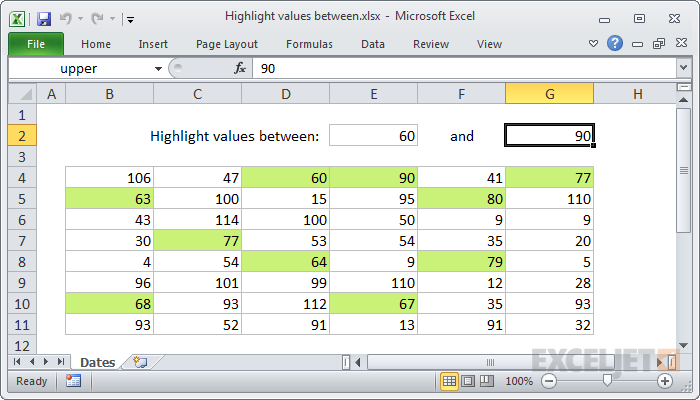
If you want to use conditional formatting to highlight cells that are "greater than X and less than Y", you can use a simple formula that returns TRUE when a value meets those conditions. For example, if you have numbers in the range B4:G11, and want to highlight cells with a numeric value over 60 and less than 90, select B4:G11 and create a conditional formatting rule that uses this formula:
=AND(B4>=60,B4<=90)
It's important that the formula be entered relative to the "active cell" in the selection, which is assumed to be B4 in this case.
Also note that we are using greater than or equal to, and less than or equal to in order to include both the lower and upper values.
Generic formula
=AND(A1>=lower,A1<=upper)
Explanation
When you use a formula to apply conditional formatting, the formula is evaluated for each cell in the range, relative to the active cell in the selection at the time the rule is created. So, in this case, if you apply the rule to B4:G11, with B4 as the active cell, the rule is evaluated for each of the 40 cells in B4:G11 because B4 is entered as a fully relative address. Because we are using AND with two conditions, the formula returns TRUE only when both conditions return TRUE, triggering the conditional formatting.
Using other cells as inputs
You don't have to hard-code the numbers into the rule and, if the numbers will change, it's better if you don't.
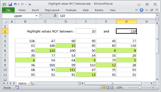
To make a more flexible, interactive conditional formatting rule, use other cells like variables in the formula. For example, if you want to use cell E2 for the lower limit, and cell G2 for the upper limit, you can use this formula:
=AND(B4>=$E$2,A1<=$G$2)
You can then change the values in cells E2 and G2 to anything you like and the conditional formatting rule will respond instantly. You must use an absolute address for E2 and G2 to prevent these addresses from changing.
With named ranges
A better way to lock these references is to use a named ranges, since named ranges are automatically absolute. If you name cell E2 "lower" and the cell G2 "upper", then you can write the conditional formatting formula like so:
=AND(B4>=lower,B4<=upper)
Named ranges allow you to use a cleaner, more intuitive syntax.