Summary
To highlight blank cells (i.e. empty cells) with conditional formatting, you can use a simple formula based on the ISBLANK function. In the example shown, the formula used to highlight blank cells is:
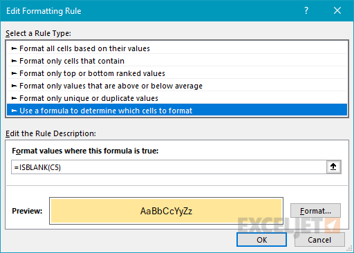
=ISBLANK(C5)
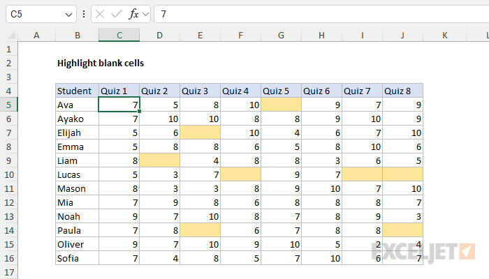
When this formula returns TRUE, it triggers a Conditional Formatting rule that applies a bright fill color to empty cells in the range C5:J16. This makes it easy to see at a glance which students are missing quiz scores. The formatting is dynamic — if the data changes, the highlighting will automatically update.
Generic formula
=ISBLANK(A1)
Explanation
In this example, the goal is to highlight empty cells in the range C5:J16 with conditional formatting. This is a quick and easy way to locate missing values in a data set. To apply a conditional formatting rule to highlight empty cells, follow these steps:
- Select the range that contains empty cells you want to highlight (C5:J16 in this case).
- On the Home tab of the ribbon, click Conditional Formatting, then New Rule.
- In the list of options for rule type, select "Use a formula to determine which cells to format".
- In the input area, add the following formula: =ISBLANK(C5)
- Click the Format button and configure the desired formatting.
The result should be a Conditional Formatting rule like this:
When you use a formula to apply conditional formatting, the formula is evaluated relative to the active cell in the selection at the time the rule is created. So, in this case, the formula =ISBLANK(C5) is evaluated for each cell in C5:J16. Because C5 is entered as a relative address, the address will be updated each time the formula is applied, and ISBLANK() is run on each cell in the range. The TRUE or FALSE result for each cell is what triggers the rule.
Empty vs. blank
The ISBLANK function only returns TRUE if a cell contains no value. If a cell contains a formula that returns an empty string (""), the result may look like an empty cell, but ISBLANK will return FALSE because the cell contains a formula. As a result, the cell won't be highlighted. If you want to highlight cells that contain an empty string ("") returned by a formula, you can use this formula instead:
=LEN(C5)=0
The LEN function returns the length of a text string as a number. A cell that contains an empty string ("") will have a length of zero, so the formula will return TRUE for cells that are truly empty and cells that contain an empty string ("") returned by a formula.
Not blank
To conditionally format cells that are not blank, you can use a formula like this:
=NOT(ISBLANK(A1))
The NOT function reverses the logic.