Summary
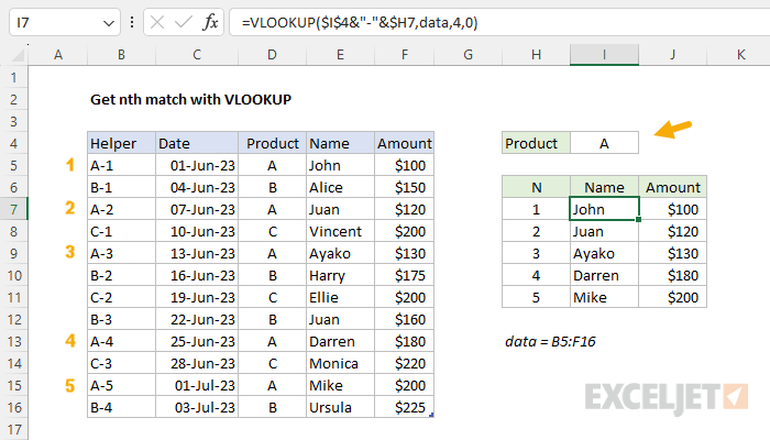
To get the nth match in a set of data with the VLOOKUP function, you can use a helper column that contains a special calculated lookup value. In the worksheet shown, the formula in cell I7 looks like this:
=VLOOKUP($I$4&"-"&$H7,data,4,0)
Where data is an Excel Table in the range B5:F16. When I4 contains "A", the formula will return the first 5 matches as it is copied down column I, using the numbers in column H for n. A similar formula can be used to return the amount associated with the nth match in cell J7. See below for details.
The purpose of this example is to explain how to get the nth match in Excel 2019 and older with VLOOKUP. It is also possible to use a formula based on INDEX and MATCH. However, in the current version of Excel, the FILTER function is a much better way to get multiple matching records.
Generic formula
=VLOOKUP(id_formula,table,n,0)
Explanation
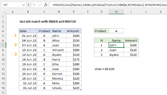
The table contains basic order information, with columns for Date, Product, Name, and Amount. The Helper column is used to create a special lookup value, as explained below. The goal is to retrieve the nth matching record in a table for a specific product, which is entered in cell I4. For example, if the value in cell H4 is "A", the formula in I7 should return the name "John", since this is the first name in the table associated with product "A". In the same way, the formula in I8 should return 'Juan', since this is the second name associated with product "A". If the product in H4 is changed, the formula should calculate a new result. All data exists in an Excel Table named data.
Helper column
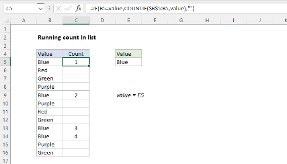
This formula depends on a helper column, which is added as the first column to the source data table. The helper column uses a formula to create a unique ID to use as a lookup value using the product in column D and a counter created with the COUNTIF function. The lookup value is created by concatenating the product in I4 to a running count of the product. The formula in B5 is:
=D5&"-"&COUNTIF($D$5:D5,D5)
This formula picks up the value in D5 and uses the ampersand (&) to concatenate the product to a hyphen (-), and the result from COUNTIF. The COUNTIF function uses an expanding range ($D$5:D5) to generate a running count of the product in the table. The values in column B show the results of this formula.
VLOOKUP function
VLOOKUP is an Excel function to get data from a table organized vertically, with lookup values in the first column. The data to retrieve is specified by column number, and the generic syntax for VLOOKUP looks like this:
=VLOOKUP(lookup_value,table_array,column_index_num,range_lookup)
In this example, we use the formulas below to look up the name and amount for each match in the table:
=VLOOKUP($I$4&"-"&$H7,data,4,0) // name
=VLOOKUP($I$4&"-"&$H7,data,5,0) // amount
The lookup_value is the value to search for, and this is the tricky part of this approach. To match the lookup values in column B, we need to create a lookup value in the same format as the IDs we created in the Helper column: a product code joined to a count, separated by a hyphen (i.e., "A-1", "A-2", etc.). To do this, we use the snippet below:
$I$4&"-"&$H7
Notice the reference to $I$4 is absolute so that it will not change when the formula is copied, while the reference to $H7 is mixed so that the column is locked but the row can change. As the formula is copied down, the lookup_value increments at each row using the numbers in column H. This is how the formula can return the first match, the second match, and so on.
The table_array is the Excel Table named data. Next, we have the column number, which is a number that indicates the column from which we want to retrieve data, where the first column is column 1 and contains lookup values. To get the Name, we use 4 for column_index_num, and to get the Amount, we use 5. Finally, we have the last argument, range_lookup, for which we provide zero (0). Using zero (0) tells VLOOKUP to find an exact match for the ID. If the exact ID isn't found, VLOOKUP will return the #N/A error.
As the VLOOKUP formulas are copied down, they return the first five matches for Product A as shown in the worksheet. In cells I7 and J7, the lookup values and results look like this:
=VLOOKUP("A-1",data,4,0) // returns "John"
=VLOOKUP("A-1",data,5,0) // returns 100
In cells I8 and J8, we have:
=VLOOKUP("A-2",data,4,0) // returns "Juan"
=VLOOKUP("A-2",data,5,0) // returns 120
And so on, as the formula is copied down.
For more information about VLOOKUP, see: How to use the VLOOKUP function.