Explanation
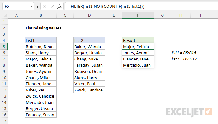
In this example, the goal is to generate a list of people who were invited but did not attend an unspecified event. More specifically, we need to compare the names in B5:B16 against the names in D5:D12 and return the missing names. For convenience, list1 (B5:B16) and list2 (D5:D12) are named ranges. The easiest way to solve this problem in Excel is with the FILTER function and the COUNTIF function, as explained below.
FILTER function
This formula uses the FILTER function to retrieve data based on a logical test built with the COUNTIF function. In the worksheet shown, the formula in cell F5 is:
=FILTER(list1,NOT(COUNTIF(list2,list1)))Working from the inside out, the COUNTIF function is used to create the actual filter:
COUNTIF(list2,list1)
Notice we are using list2 as the range argument, and list1 as the criteria argument. In other words, we ask COUNTIF to count all values in list1 that appear in list2. Because we are giving COUNTIF multiple values for the criteria, we get back an array with multiple results:
{1;1;0;1;0;1;0;1;1;0;1;1}Note that the array contains 12 counts, one for each value in list1. Also, notice that there are 4 zeros in the array. A zero value indicates a name in list1 that was not found in list2. The 1's in the array indicate a name in list1 that was found in list2. Because we want to list names that did not attend, we deliver the result from COUNTIF to the NOT function:
NOT({1;1;0;1;0;1;0;1;1;0;1;1})The NOT function effectively reverses the result from COUNTIF. Any non-zero number becomes FALSE, and any zero value becomes TRUE. The result from NOT is an array like this:
{FALSE;FALSE;TRUE;FALSE;TRUE;FALSE;TRUE;FALSE;FALSE;TRUE;FALSE;FALSE}Notice there are now 4 TRUE values in the array. This is what we need to report the missing names. The array is returned directly to the FILTER function as the include argument, and the FILTER function uses the array as a filter. The result is an array of 4 missing names that land in cell F5 and spill into the range F5:F8. If any data changes, FILTER will recalculate and return an updated list.


