Filter values within tolerance

In this example, the goal is to list values in a given group that are within a given tolerance. The group is set in cell G4, and the target value is entered in cell G5. The allowed tolerance is entered in cell G6. The data comes from an Excel Table called data in the range B5:D16. The solution is built on the FILTER function which can be used to extract and list data that meets multiple criteria. The beauty of this formula is that tolerance calculations do not need to be in the source data. The FILTER function creates the data it needs on the fly. When any of the variable inputs in G5:G6 are changed, or if source data changes, the results update immediately.

Background reading

This article assumes you are familiar with Excel Tables and the FILTER function. If not, see:

• Excel Tables - introduction and overview
• Value is within tolerance - formula example
• The FILTER function - introduction and overview
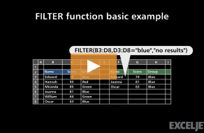
• Basic FILTER function example (video)
• Dynamic Array Formulas (paid training)

Filter by Group

In order to extract records where the group is "A", we can use FILTER like this:

=FILTER(data,data[Group]="A") // group A only

Here, the array argument is the entire table, since we want both columns in the output. The include argument is supplied as a simple logical expression that returns TRUE or FALSE for each value in the Group column:

data[Group]="A" // returns TRUE or FALSE

Because we want the group to be a variable input, we need to replace the hardcoded text string "A" with a reference to cell G4, which allows the user to change the group as desired:

=FILTER(data,data[Group]=G4)

Now when a user types "B" into cell G4, FILTER will extract all values from group B.

Values within tolerance

The next task in the formula is to test for values within a given tolerance, where the target value comes from cell G5, and the acceptable tolerance is defined in cell G6. The generic logical expression for this test looks like this:

ABS(value-target)<=tolerance)

The ABS function is used to convert negative differences to positive values. See this formula for a more detailed explanation. Mapping the cell references in the example to the generic formula, we get this logical expression:

ABS(data[Value]-G5)<=G6)

This expression will return TRUE or FALSE for each number in the Value column. To extract all values within tolerance, ignoring group, we can use the expression above as the include argument in FILTER:

=FILTER(data,ABS(data[Value]-G5)<=G6) // ignore group

FILTER will ignore group and return all values within tolerance.

Combining expressions

Now we need to combine both logical conditions above into a single formula. For this, we use Boolean logic. Because we want to join the two expressions with AND (i.e. we want to enforce both conditions) we use the multiplication operator between the expressions like this:

=(data[Group]=G4)*(ABS(data[Value]-G5)<=G6)

Each expression generates its own array of TRUE and FALSE values, and the multiplication operation automatically coerces the TRUE and FALSE values to 1s and 0s. The standalone formula above will return 1 for values that meet both conditions, and 0 for other values.

Video: Boolean algebra in Excel

Finally, we need to place the expression into the FILTER function as the include argument:

=FILTER(data,(data[Group]=G4)*(ABS(data[Value]-G5)<=G6))

This is the final formula. With "A" in G4, 1.2 in G5, and 0.05 in G6, the FILTER function returns rows in the table where values in Group A are within +/- 0.05 of 1.2. These results are returned to cell F9 and spill onto the worksheet. If any of the variable inputs in G4:G6 are changed, results are immediately updated.

Filter on values out of tolerance

To reverse the logic explained above to show values that are out of tolerance, simply change the logical operator in the tolerance expression from less than or equal to (<=), to greater than (>):

=FILTER(data,(data[Group]=G4)*(ABS(data[Value]-G5)>G6))

The screen below shows the result: