Count paired items in listed combinations

To build a summary table with a count of paired items that appear in a list of existing combinations, you can use a helper column and a formula based on the COUNTIFS function. In the example shown the formula in cell H5 is:

=IF($G5=H$4,"-",COUNTIFS(helper,"*"&$G5&"*",helper,"*"&H$4&"*"))

where helper is the named range E5:E16.

Note: this formula assumes items don't repeat in a given combination (i.e. AAB, EFE are not valid combinations).

Explanation

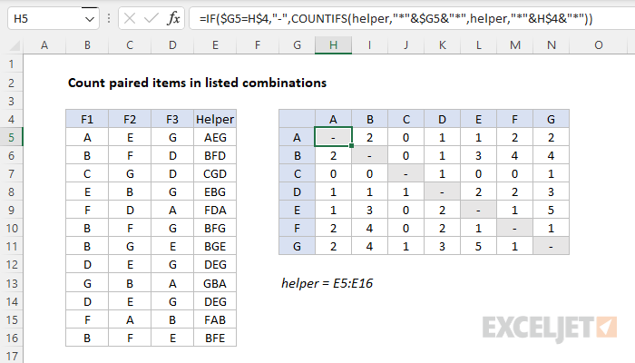
We want to count how often items in columns B, C, and D appear together. For example, how often A appears with C, B appears with F, G appears with D, and so on. This would seem like a perfect use of COUNTIFS, but if we try to add criteria looking for 2 items across 3 columns, it isn't going to work.

A simple workaround is to join all items together in a single cell in a helper column, then use COUNTIFS with a wildcard to count items. We do that with a helper column (E) that joins items in columns B, C, and D using the CONCAT function. The formula in E5, copied down, is:

=CONCAT(B5:D5)

As an alternative, you can also manually concatenate the values like this:

=B5&C5&D5

Because repeated items are not allowed in a combination, the first part of the formula excludes matching items. If the two items are the same, the formula returns a hyphen or dash as text:

=IF($G5=H$4,"-"

If items are different, a COUNTIFS function is run:

COUNTIFS(helper,"*"&$G5&"*",helper,"*"&H$4&"*")

Here, the COUNTIFS function is configured to count "pairs" of items. Only when corresponding values from column G and row 4 appear together in the helper column is the pair counted. Because a letter may appear anywhere, the asterisk (*) wildcard is concatenated to both sides of the value to ensure a match will be counted no matter where it appears in the cell. Note the references to G5 and H4 are mixed references in order to lock the column and row as needed when the formula is copied across the table.