Summary
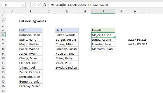
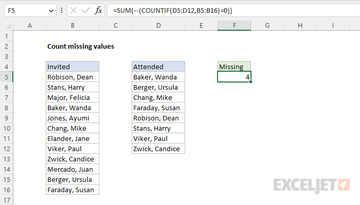
To count the values in one list that are missing from another list, you can use a formula based on the COUNTIF function. In the example shown, the formula in F5 is:
=SUM(--(COUNTIF(D5:D12,B5:B16)=0))
This formula returns 4 because there are 4 names in B5:B16 that are missing from D5:D12.
Note: In the current version of Excel, the SUM function "just works" with no special handling. In Legacy Excel, this is an array formula that must be entered with control + shift + enter. To avoid this requirement, you can replace the SUM function with the SUMPRODUCT function.
Generic formula
=SUM(--(COUNTIF(list2,list1)=0))
Explanation
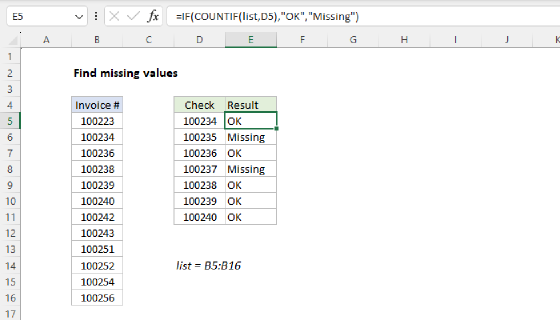
In this example, the goal is to count the number of names in the range B5:B16 (Invited) that are missing from the range D5:D12 (Attended). This problem can be solved with the COUNTIF function or the MATCH function, as explained below. Both approaches work well. The advantage of the MATCH approach is that it will work with arrays or ranges. The COUNTIF function is limited to ranges only, like other functions in this group.
COUNTIF solution
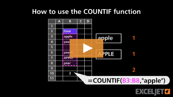
The COUNTIF function counts cells that meet a single condition, which is referred to as "criteria". The generic syntax for COUNTIF looks like this:
=COUNTIF(range,criteria)
For example, to count the cells in A1:A10 that are equal to "apple", you could use COUNTIF like this:
=COUNTIF(A1:A10,"apple")
In this example, we are doing something interesting. We are giving COUNTIF more than one value to count, supplied in the range B5:B16, and we are asking COUNTIF to count these values in the range D5:D12:
=COUNTIF(D5:D12,B5:B16)
Literally, this formula means "count the values in B5:B16 that appear in D5:D12". Because we are giving COUNTIF a range that contains 12 values, COUNTIF returns 12 results in an array like this:
{1;1;0;1;0;1;0;1;1;0;1;1}
The 1s in this array signify names in B5:B16 that appear in D5:D12. The 0s indicate names in B5:B16 that don't appear in D5:D12. If the goal was to count matching values, we could sum the result from COUNTIF with the SUM function like this:
=SUM(COUNTIF(D5:D12,B5:B16)) // returns 8
The result would be 8 since there are 8 names in B5:B16 that appear in D5:D12. However, in this problem, the goal is to count missing values, so we need to "reverse" the result from COUNTIF before we sum. In other words, we need to convert the 1s to 0s and the 0s to 1s. We can do that by first comparing the result from COUNTIF to zero:
COUNTIF(D5:D12,B5:B16)=0
This will result in an array with 12 TRUE and FALSE values like this:
{FALSE;FALSE;TRUE;FALSE;TRUE;FALSE;TRUE;FALSE;FALSE;TRUE;FALSE;FALSE}
Notice that in this array, the FALSE values correspond to 1s in the previous array, and the TRUE values correspond to 0s. If we try to add these values up with the SUM function, the result will be zero, because SUM is programmed to ignore the logical values TRUE and FALSE. Before we sum, we need to convert the TRUE and FALSE values to 1s and 0s again. We do that with a double negative (--) operation:
--(COUNTIF(D5:D12,B5:B16)=0) // returns {0;0;1;0;1;0;1;0;0;1;0;0}
The result is a numeric array:
{0;0;1;0;1;0;1;0;0;1;0;0}
In this array, 0s represent names in B5:B16 that appear in D5:D12, and 1s represent missing names. This array is returned directly to the SUM function, and SUM returns 4 as a final result:
=SUM({0;0;1;0;1;0;1;0;0;1;0;0}) // returns 4
Note: In the current version of Excel, the SUM function works without special handling. In Legacy Excel, this is an array formula and must be entered with control + shift + enter. To avoid this requirement, you can replace SUM with SUMPRODUCT, and control + shift + enter is not required.
MATCH solution
Another way to solve this problem in a more literal way is to use the MATCH function to match names. The MATCH function returns the position of a value in a range. For example, if the range A1:A3 contains "orange", "apple", and "pear", then the MATCH function will return 2 if we look for "apple", because "apple" appears in the 2nd cell:
=MATCH("apple",A1:A3,0) // returns 2
If we look for a value that does not exist in the range, MATCH will return an #N/A error:
=MATCH("banana",A1:A3,0) // returns #N/A
We can use the behavior above to solve the problem in this example with a formula like this:
=SUM(--ISNA(MATCH(B5:B16,D5:D12,0)))
Working from the inside out, MATCH is configured to match the values in B5:B16 against the values in D5:D12:
MATCH(B5:B16,D5:D12,0)
Note that the value for match_type is zero (0) to specify an exact match. Like the COUNTIF formula above, we are asking MATCH to look for the values in B5:B16 (Invited) in the values in D5:D12 (attended). Because we are looking for 12 values, MATCH will return an array with 12 results like this:
{5;6;#N/A;1;#N/A;3;#N/A;7;8;#N/A;2;4}
In this array, numbers represent the position of a name that was found, and #N/A errors represent names that were not found. This array is returned directly to the ISNA function:
ISNA({5;6;#N/A;1;#N/A;3;#N/A;7;8;#N/A;2;4})
ISNA returns TRUE for #N/A errors and FALSE for anything else, so the result from ISNA looks like this:
{FALSE;FALSE;TRUE;FALSE;TRUE;FALSE;TRUE;FALSE;FALSE;TRUE;FALSE;FALSE}
As with the COUNTIF formula, we want to count these results, but we first need to convert the TRUE and FALSE values to 1s and 0s. We do this with a double negative (--) operation:
=SUM(--{FALSE;FALSE;TRUE;FALSE;TRUE;FALSE;TRUE;FALSE;FALSE;TRUE;FALSE;FALSE})
=SUM({0;0;1;0;1;0;1;0;0;1;0;0})
=4
The final result is 4 since there are 4 names in B5:B16 that do not appear in D5:D12.
Note: One advantage of the MATCH function is that it will work with data in arrays or ranges, while the COUNTIF function is limited to ranges only.