Summary
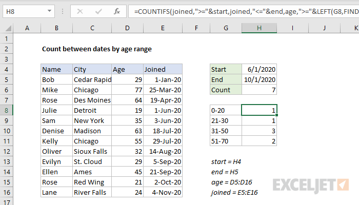
To count values between two dates that also fall into specific numeric ranges, you can use a formula based on the COUNTIFS function, with help from the LEFT, RIGHT, FIND, and LEN functions. In the example shown the formula in H8, copied down, is:
=COUNTIFS(joined,">="&start,joined,"<="&end,
age,">="&LEFT(G8,FIND("-",G8)-1),
age,"<="&RIGHT(G8,LEN(G8)-FIND("-",G8)))
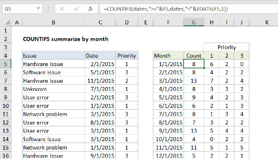
where start (H4), end (H5), age (D5:D16), and joined (E5:E16) are named ranges. At each new row, the formula returns the count of all rows between start and end dates (inclusive) that also fall into the age ranges shown in column G.
Note: this is a somewhat advanced formula that demonstrates how the criteria for COUNTIFS can be extended, and quite a lot of the complexity comes from having to parse the age ranges in column G. If you just want to count things between two dates, this formula is more straightforward.
Explanation
The goal of this example is to count rows in the data where the date joined falls between start and end dates (inclusive) and the age also falls into the age ranges seen in column G. The formula is complicated somewhat by the fact that the age range labels are actually text, so we need to extract a low and high number for each age range as a separate step.
Note: the named ranges shown in this example are entirely optional. They are a way to make the formula easier to enter, read, and copy.
Count between dates
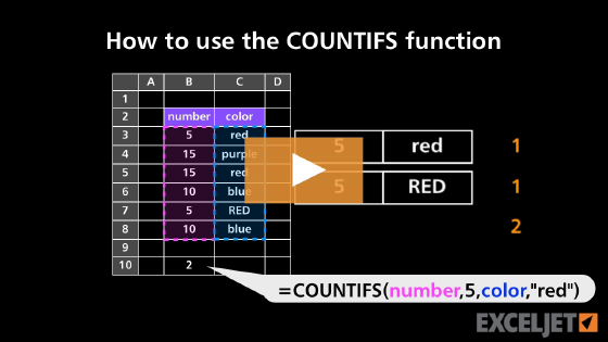
The main function used to solve this problem is COUNTIFS. To explain how this works, we'll look first at the total seen in cell H6. This total does not take into account age groups, it simply counts all records that fall between the start and end dates. The formula in H6 is:
=COUNTIFS(joined,">="&start,joined,"<="&end)
COUNTIFS is configured with two range/criteria pairs: one to count join dates greater than or equal to the start date in cell H4:
joined,">="&start // greater than or equal to start
and one to count join dates less than or equal to the end date in cell H5:
joined,"<="&end // less than or equal to end
Note that we are concatenating the operators inside the formula with the ampersand (&). The COUNTIFS function belongs to a group of functions that use this syntax.
With this configuration, COUNTIFS returns the total records with a join date greater than or equal to the start and end dates in H4 and H5.
Count between age range
The formula above counts records using the start and end dates, but does not take age range into account. To further restrict the count to the age ranges shown in column G, we need to add two more range/criteria pairs. The first pair restricts the count to ages greater than or equal to the "low" number:
age, ">="&LEFT(G8,FIND("-",G8)-1) // low
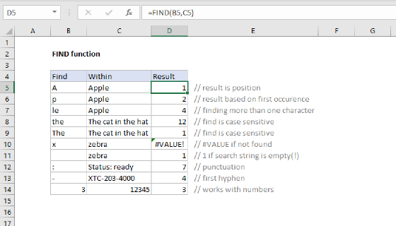
Here, we use the FIND and LEFT function to extract the low number. The FIND function returns the position of the hyphen (-) and feeds this number (minus 1) to the LEFT function as the number of characters to extract. LEFT returns zero ("0"), which is concatenated to the greater than or equal to operator (>=). In the end, we have:
age,">=0"
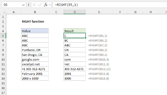
The second range/criteria pair restricts the count to ages less than or equal to the "high" number in the age range:
age,"<="&RIGHT(G8,LEN(G8)-FIND("-",G8)) // high
As before, we use the FIND function to locate the position of the hyphen (-). The result is subtracted from the total of all characters in the cell (calculated with the LEN function) and this result is given to the RIGHT function for the number of characters to extract from the right side. RIGHT returns 20, which is concatenated to the less than or equal to operator (<=). In the end, we have:
age,"<=20"
As this formula is copied down the range H8:H11, the high and low values in the age ranges are extracted and used as conditions to restrict the count , while the original date logic remains unchanged.
With SUMPRODUCT
This problem can also be solved with the SUMPRODUCT function. To get the total in cell H6, you can use a formula like this:
=SUMPRODUCT((joined>=start)*(joined<=end))
To count by age ranges, the formula in H8, copied down, is:
=SUMPRODUCT((joined>=start)*(joined<=end)*(age>=LEFT(G8,FIND("-",G8)-1)+0)*(age<=RIGHT(G8,LEN(G8)-FIND("-",G8))+0))
Note when checking the age, we need to add zero to the result from the LEFT function and the RIGHT function, because these functions return text, and any text value will cause the age checks to fail. Adding zero is an easy way to convert a number represented as text into a true numeric value. This isn't necessary with COUNTIFS above, because COUNTIFS does some kind of internal magic to evaluate numeric criteria correctly, even though the criteria is provided as text.
TEXTBEFORE and TEXTAFTER
The new TEXTBEFORE and TEXTAFTER functions can help simplify the formulas above, because they make it easier to parse the age range. The COUNTIFS version can be simplified to:
=COUNTIFS(joined,">="&start,joined,"<="&end,age,">="&TEXTBEFORE(G8,"-"),age,"<="&TEXTAFTER(G8,"-"))
And the SUMPRODUCT version can be written as:
=SUMPRODUCT((joined>=start)*(joined<=end)*(age>=TEXTBEFORE(G8,"-")+0)*(age<=TEXTAFTER(G8,"-")+0))
TEXTBEFORE and TEXTAFTER are currently available in Excel 365 only.