Summary
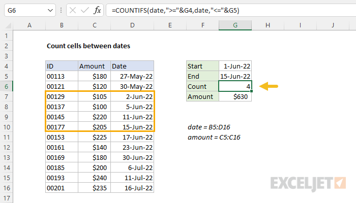
To count the number of cells that contain dates between two dates, you can use the COUNTIFS function. In the example shown, G6 contains this formula:
=COUNTIFS(date,">="&G4,date,"<="&G5)
where date is the named range D5:D16. The result is the number of dates in D5:D16 that are between June 1, 2022 and June 15, 2022, inclusive.
Generic formula
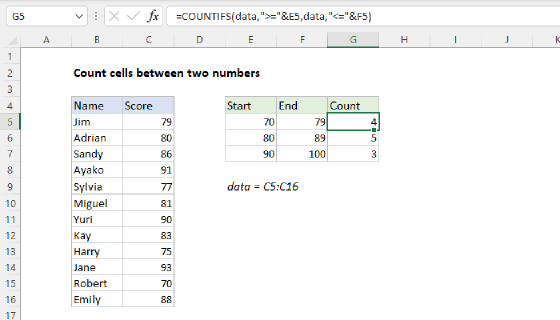
=COUNTIFS(range,">="&date1,range,"<="&date2)
Explanation
In this example, the goal is to count the number of cells in column D that contain dates that are between two variable dates in G4 and G5. This problem can be solved with the COUNTIFS function or the SUMPRODUCT function, as explained below. For convenience, the worksheet contains two named ranges: date (D5:D16) and amount (C5:C16). The named range amount is not used to count dates, but can be used to sum amounts between the same dates, as seen below.
Note: Excel dates are large serial numbers so, at the core, this problem is about counting numbers that fall into a specific range. In other words, SUMIFS and SUMPRODUCT don't care about the dates, they only care about the numbers underneath the dates. If you like, you can see the numbers underneath by temporarily formatting the dates with the General number format.
COUNTIFS function
The COUNTIFS function is designed to count cells that meet multiple conditions. In this case, we need to provide two conditions: (1) the date is greater than or equal to G4 and (2) the date is less than or equal to G5. COUNTIFS accepts conditions as range/criteria pairs, so the conditions are entered like this:
date,">="&G4 // greater than or equal to G4
date,"<="&G5 // less than or equal to G5
The final formula looks like this:
=COUNTIFS(date,">="&G4,date,"<="&G5)
Note that the logical operators ">=" and "<=" must be entered as text and surrounded by double quotes. This means we must use concatenation with the ampersand operator (&) to join the operators to the dates in cell G4 and cell G5. This syntax is specific to a group of eight functions in Excel.
SUMPRODUCT function
This problem can also be solved with the SUMPRODUCT function which allows a cleaner syntax:
=SUMPRODUCT((date>=G4)*(date<=G5))
This is an example of using Boolean algebra in Excel. Because the named range date contains 12 dates, each expression inside SUMPRODUCT returns an array with 12 TRUE or FALSE values. When these two arrays are multiplied together, they return an array of 1s and 0s. After multiplication, we have:
=SUMPRODUCT({0;0;1;1;1;1;0;0;0;0;0;0})
SUMPRODUCT then returns the sum of the elements in the array, which is 4.
Sum amounts between dates
To sum the amounts on dates between G4 and G5 in this worksheet, you can use the SUMIFS function like this:
=SUMIFS(amount,date,">="&G4,date,"<="&G5)
The conditions in SUMIFS are the same as in COUNTIFS, but SUMIFS also accepts the range to sum as the first argument. The result is $630.
To sum the amounts for dates between G4 and G5, you can use SUMPRODUCT like this:
=SUMPRODUCT((date>=G4)*(date<=G5)*amount)
Here again, the conditions are the same as the original SUMPRODUCT formula above, but we have extended the formula to multiply by amount. This formula simplifies to:
=SUMPRODUCT({0;0;1;1;1;1;0;0;0;0;0;0}*{180;120;105;100;220;205;225;140;180;200;240;235})
The zeros in the first array effectively cancel out the amounts for dates that don't meet criteria:
=SUMPRODUCT({0;0;105;100;220;205;0;0;0;0;0;0})
and SUMPRODUCT returns $630 as a final result.